Vertex AI Tutorial: A Comprehensive Guide For Beginners

Even though most people associate Google with search engines, the company also has deep roots in the data science industry. It consistently delivers state-of-the-art products and solutions aimed at getting the most benefit from data. One of their products, Vertex AI, was released in 2021 to simplify the machine learning process at an enterprise scale.

In this tutorial, we will learn how to get started with Google’s Vertex AI platform and how to use it to cover a wide range of tasks of the ML life cycle. We will leave with a deployed model we can use to send requests to generate predictions for a classification task.

What is Vertex AI?

A typical machine learning life cycle consists of many stages:

• Data preparation, ingestion, exploration
• Feature engineering, selection
• Model training and tuning
• Deploying and model monitoring

All these stages and substages require a different set of tools and diverse team of experts to coordinate them.

Vertex AI by Google Cloud streamlines and unifies this entire process into a single platform.

While large-scale ML applications require seasoned specialists, Vertex AI empowers users of any skill level:

• AutoML for beginners: Requires no coding experience. Simply feed in your data, and with a few clicks, AutoML generates a high-quality model for you. All the heavy lifting of data preparation, model building including algorithm selection and hyperparameter tuning is performed under the hood.
• Custom model training for experts: Your experience is the limit. For experienced data scientists and ML engineers, Vertex AI provides the flexibility to train models using their preferred frameworks, such as PyTorch, TensorFlow, or XGBoost.
• Deployment for everyone: Once you have a model trained by either AutoML or a custom one, Vertex AI makes deploying them a breeze. You can publish models as real-time APIs to integrate into your products or use batch-prediction for large-scale tasks.

There are many things we aren’t mentioning in this section, as you will get to work on most of them yourself in this tutorial.

What are Google Cloud Services?

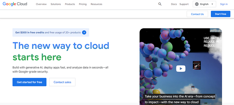
Before we start exploring the platform, we need to mention its parent — Google Cloud services. Google Cloud Services includes a wide range of cloud computing solutions that provide storage, networking, databases, analytics, and machine learning capabilities.

These services work together in sync with Vertex AI to unify your machine learning workflow. Here’s a breakdown of the services often used with Vertex AI:

Data storage and management

• Cloud storage: Acts as the central repository for your raw data, accessible by Vertex AI for training and analysis.
• BigQuery: A powerful data warehouse for storing and querying large datasets, enabling Vertex AI to use BigQuery ML for in-suite training.

Compute resources

• Compute engine: Provides virtual machines with various configurations for your custom model training needs. Vertex AI can hook up to these machines for resource-intensive training tasks.
• Vertex AI pipelines: Coordinates complex ML workflows across various compute resources for efficiency.

Google Cloud services are always available from your Google account if you visit cloud.google.com. If you have never used them before, click “Get started for free” to earn your free trial.

Otherwise, you can directly go to console.cloud.google.com so that we can get started.

Setting up your Google Cloud Console For Vertex AI

Disclaimer: If you want to follow along with the tutorial, be prepared to spend $25-30 on Vertex AI. We will be using the cheapest configurations.

When you visit your Google Cloud Console, you will most likely end up on the following welcome page:

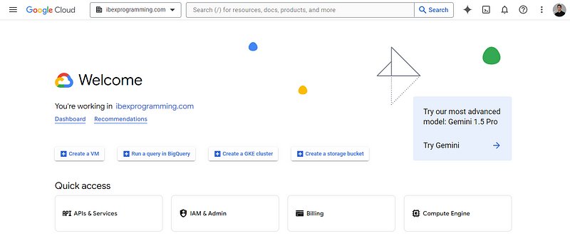
It lists your workspace name; mine is ibexprogramming.com.

The first thing we will do is to create a project. Google Cloud projects are high-level organization units for managing resources for a specific task. Here is a GIF on how to create one:

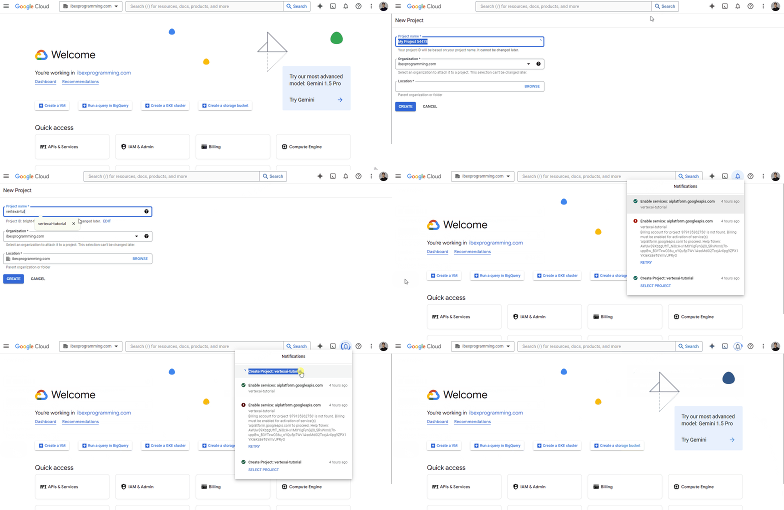
Once you the project has been created, select it so that the top bar of the page shows this:

Now, you need to create a billing account because Vertex AI requires billing information to enable its services. Don’t worry — you won’t be charged until you use paid resources. So, head over to https://console.cloud.google.com/billing:

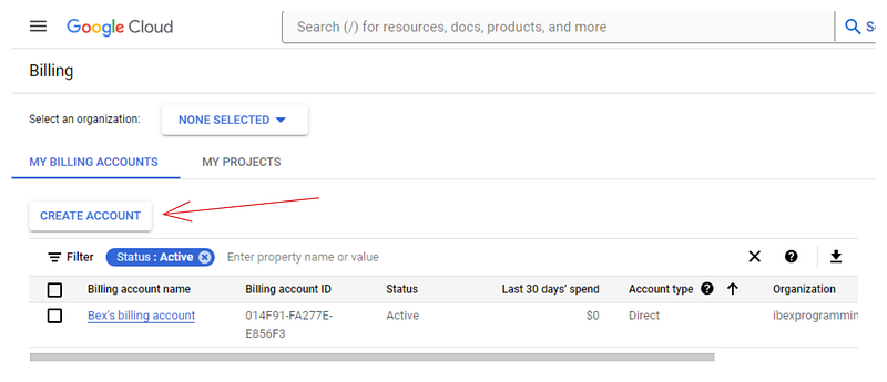
If you don’t already have an account like mine, click on “Create account” and follow the instructions shown. We will link this billing account to ours in the next section.

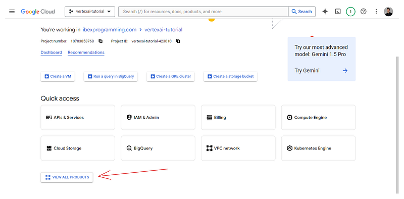
Afterward, go back to https://console.cloud.google.com/ and click on “View all products” button at the bottom of the page:

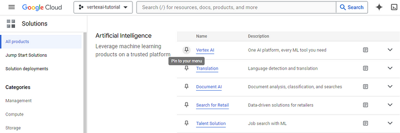
The next page will list all the services offered by Google Cloud for your project. Search for “Vertex AI” (Ctrl + F) and pin it to your menu for easy access. Then, click on the service itself:

This will direct you to your Vertex AI dashboard. A window may pop up asking you to enable Vertex AI API — choose “Enable.” If the window doesn’t pop, up you can click on the “Enable all API permissions” button to do the same.

Now, we are ready to upload a dataset to Vertex AI.

Uploading a Dataset in Vertex AI

There are a variety of ways of adding a dataset to Vertex AI. In this section, we will use a local CSV file for simplicity.

Download a sample dataset

For the article, we will be using the Dry Bean dataset from the UCI Machine Learning repository. It contains 13k instances of beans and their 15 numeric measurements.

The task is to classify them into seven types of beans: Seker, Barbunya, Bombay, Cali, Dermosan, Horoz and Sira.

After downloading, save the Excel file inside the downloaded ZIP to your local directory:

from pathlib import Path

cwd = Path.cwd()
data_path = cwd / "data" / "Dry_Bean_Dataset.xlsx"

Then, we can read this file with pandas and save it back as a CSV:

import pandas as pd

beans = pd.read_excel(data_path)

beans.shape

(13611, 17)

Note that read_excel function requires you to install the openpyxl library with PIP.

Great, we have the dataset as a DataFrame. Let’s save it back as a CSV:

beans.to_csv(cwd / "data" / "dry_bean.csv", index=False)

Create a cloud storage bucket

As we mentioned earlier, we need a Google Storage Bucket to store our raw data. Follow the GIF below to navigate to the product’s dashboard:

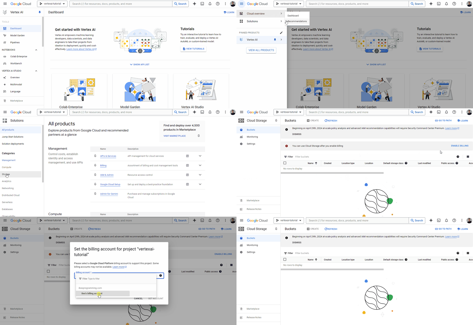
The GIF shows that to start using storage services, we need to link a billing account, which we do using the one we created earlier. Then, you will be able to create a bucket with a globally unique name:

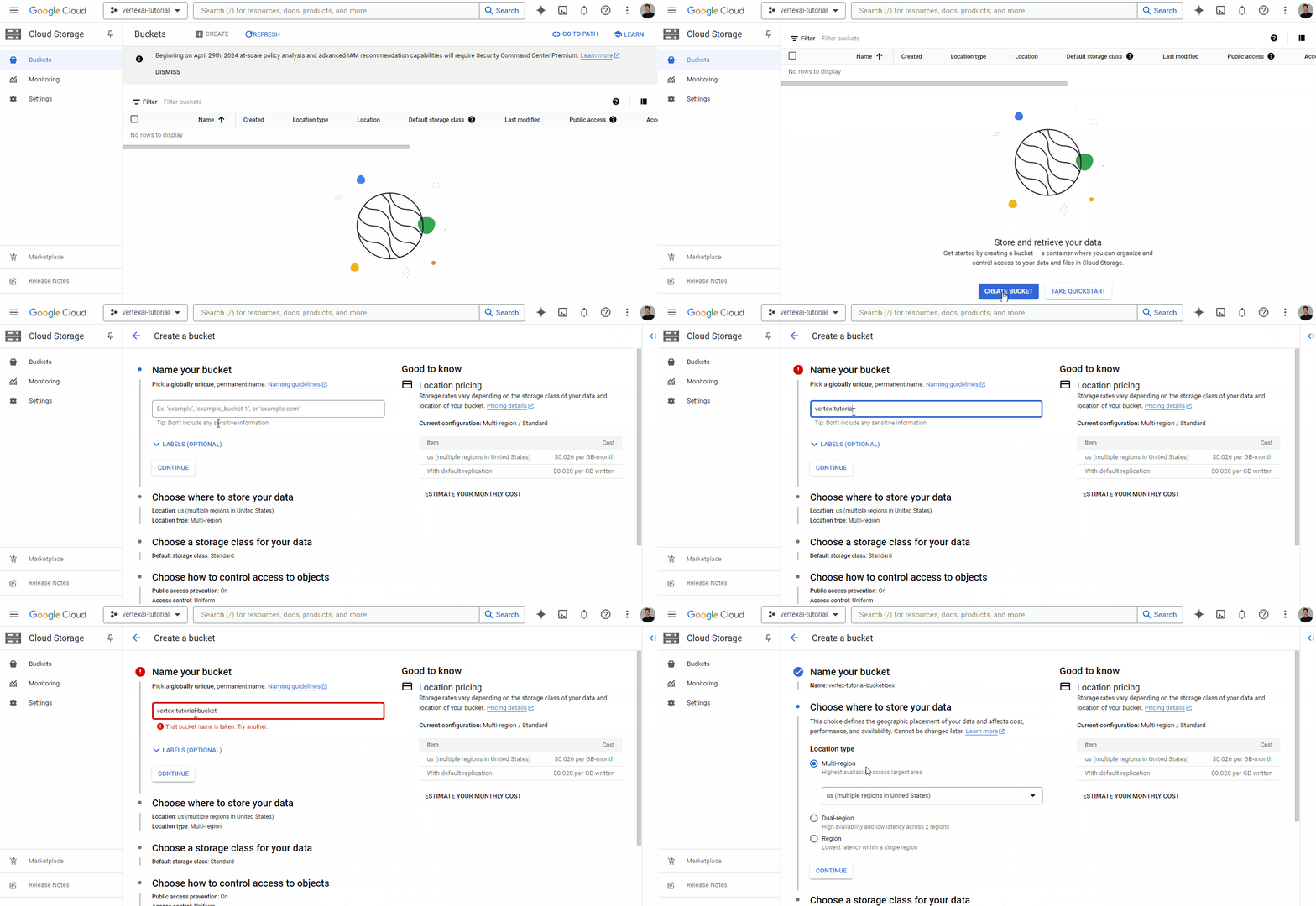
Once you find a unique name, click “Continue” until the bucket is created — you can choose default options for all fields.

Now, we are ready to ingest the CSV file we’ve saved in the previous section.

Ingest a local CSV into Vertex AI

Now, let’s move back to our Vertex AI dashboard and check out the Datasets tab:

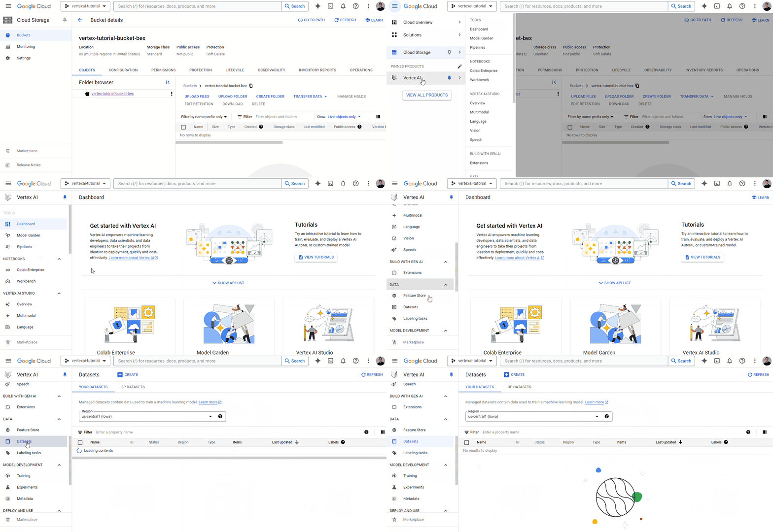
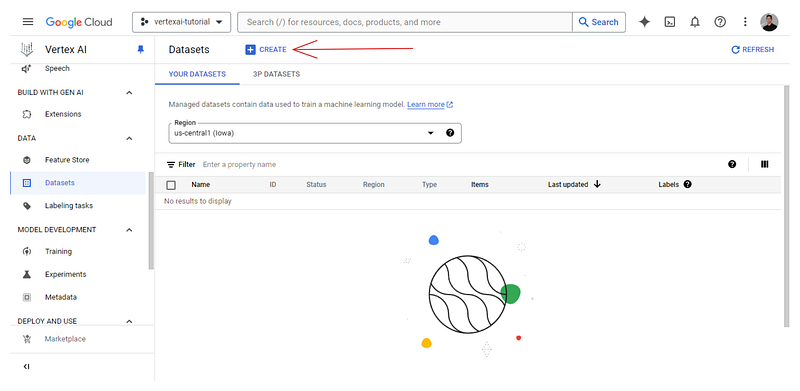
You will find it empty, so click on the “+Create” button:

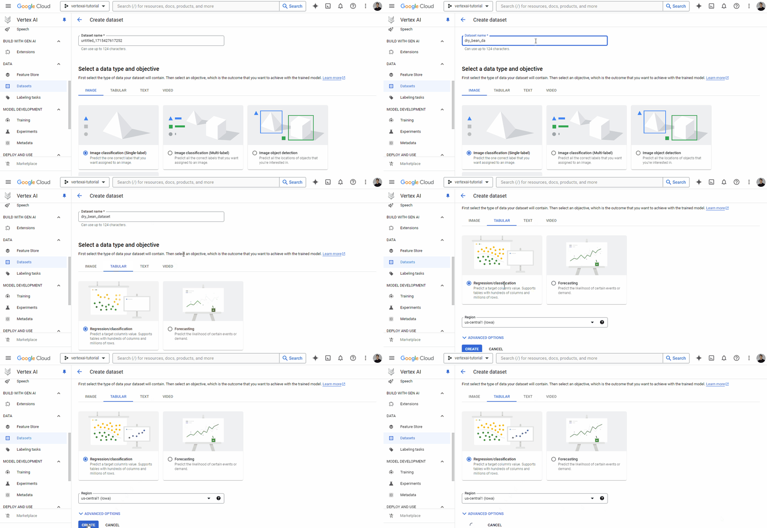
Give the dataset a unique name and choose the tabular option:

Then, the platform shows you source options. Choose to upload a local CSV file, and for the Cloud Storage path, choose the bucket you just created:

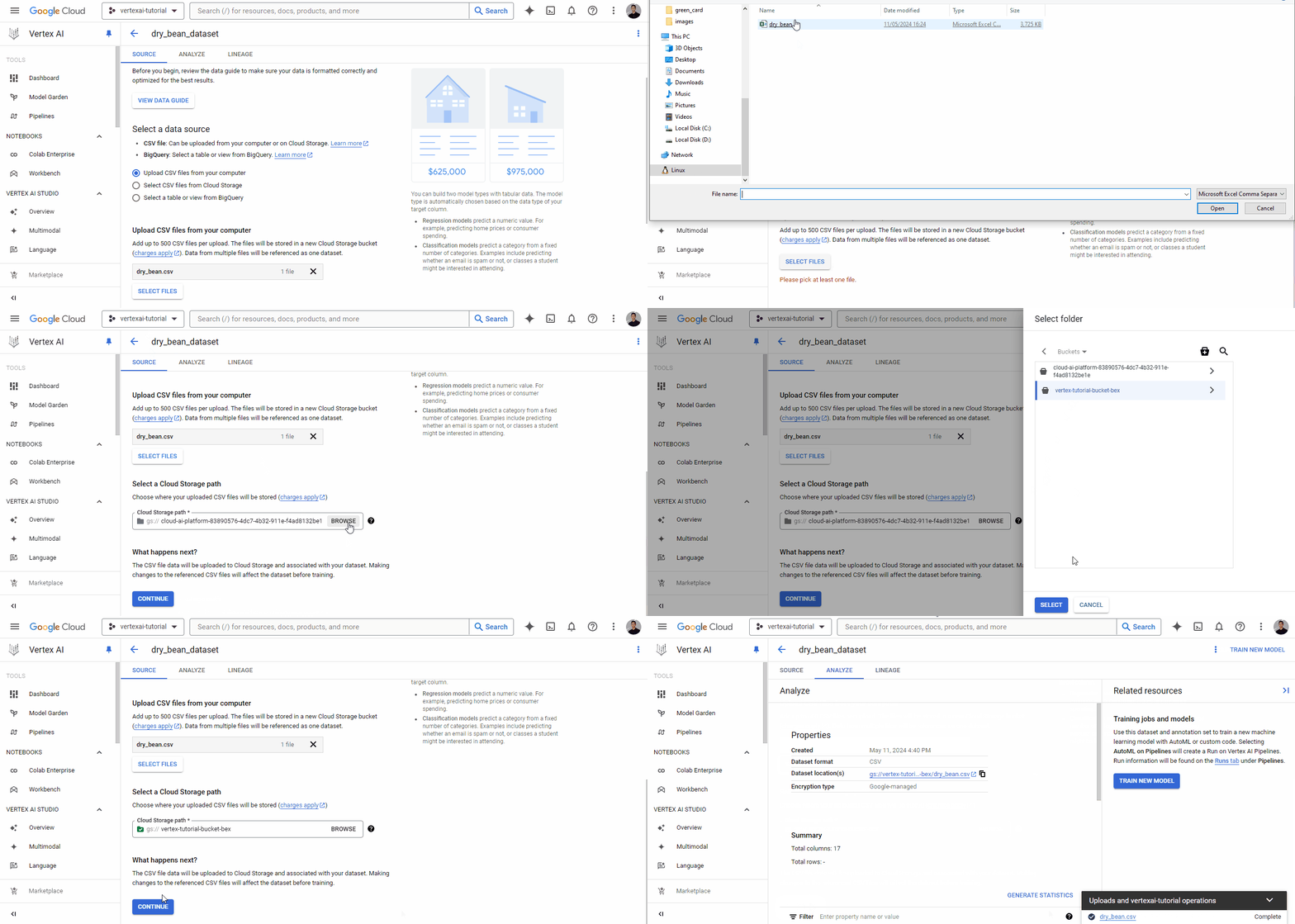
Once the dataset is successfully uploaded, you will be shown the “Analyze” tab, which shows basic metadata about the CSV file. You will also see a “TRAIN NEW MODEL” button, which will launch an AutoML training job.

However, we won’t be using that button as it’s for complete ML beginners. Instead, we will be using Vertex AI Workbench to configure a Jupyterlab coding environment and compute resources to run both AutoML and custom libraries.

Configuring Jupyterlab and Compute Resources in Vertex AI Workbench

Since Vertex AI is a unified platform, it also offers development environments called workbenches. To create a workbench, go to its own tab and follow the instructions in the GIF below:

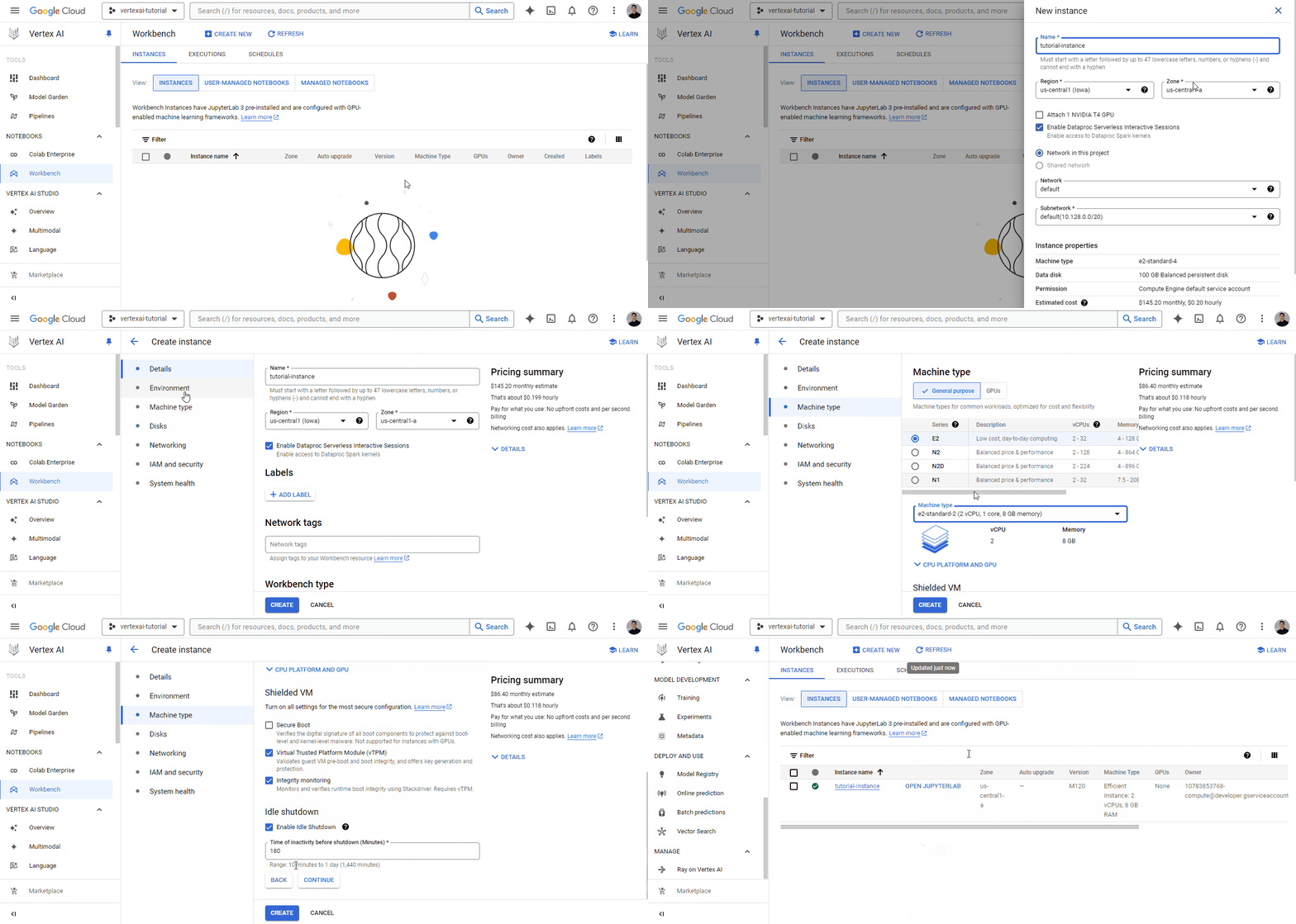
Each workbench comes with Jupyterlab 3 pre-installed. So, you only have to configure the hardware options based on your budget and needs. Since we have a pretty small dataset, I chose the weakest instance for illustration, which costs only ~0.12$ an hour (I recommend choosing a machine with more CPU cores to make computations faster).

I also changed the idle shutdown duration to 10 minutes so that the environment automatically stops if I forget to switch it off.

The workbench will take some time to initialize. Once it does, the “OPEN JUPYTERLAB” button appears, and we can click on it:

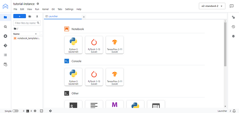
We will be directed to the familiar Jupyterlab interface. From there, create a new Python 3 notebook and rename it to whatever you want. In the first cell, install/upgrade Google Cloud services SDK google-cloud-aiplatform:

!pip3 install --upgrade --quiet google-cloud-aiplatform

Then, you can list the projects available under your account with gcloud config list:

!gcloud config list

[compute]
region = us-central1
[core]
account = # HIDDEN #
disable_usage_reporting = True
project = vertexai-tutorial-423010
[dataproc]
region = us-central1

Your active configuration is: [default]

gcloud and gsutil are both terminal utilities available in all workbenches. They allow you to manage your Google Cloud services efficiently.

From the printed output, save the following information as Python variables:

PROJECT_ID = 'vertexai-tutorial-423010'
BUCKET_URI = 'gs://vetex-tutorial-bucket-bex'
REGION = 'us-central1'

Don’t forget to change BUCKET_URI to your own bucket name. Then, import the aiplatform submodule and initialize it:

from google.cloud import aiplatform as ai

ai.init(project=PROJECT_ID, location=REGION, staging_bucket=BUCKET_URI)

aiplatform will serve as an SDK to interact with Vertex AI features.

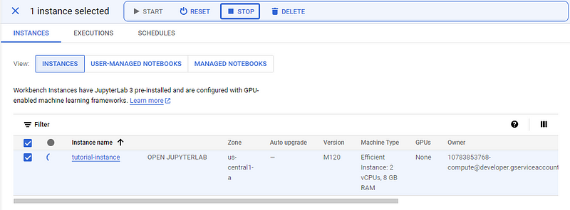
When you finish following the tutorial or take a break, don’t forget to STOP the instance to prevent unwanted costs.

Training and Deploying AutoML Models in Vertex AI

Now, let’s train a model with AutoML, which, as we mentioned earlier, takes care of all the heavy lifting for us and returns the best model it could train for the given dataset. This means that to fully take advantage of AutoML, you must ensure the dataset you are feeding to is as high-quality as possible. So, it is worth taking some time to engineer new features and perform any preprocessing steps beforehand.

AutoML preprocesses the dataset internally, but it can’t fix all the issues with your dataset.

However, in this section, we will only train a baseline AutoML model with no preprocessing or feature engineering for simplicity.

Loading data from a Google Storage bucket

The first thing we want to do is load the CSV dataset from our bucket and spend some time exploring it. Remember, EDA is an important step, and you can learn more in our Exploratory Data Analysis in Python course!

import pandas as pd

# Path to your CSV file in GCS bucket
gcs_path = "gs://vertex-tutorial-bucket-bex/dry_bean.csv"

beans = pd.read_csv(gcs_path)

beans.head()

The good news is that pandas can download files from GCS paths. The only catch is that the above code only works in Vertex AI workbenches as they are already authenticated with your Google Cloud credentials.

Exploring data with pandas in Vertex AI

We won’t perform a deep analysis of the dataset as it will distract us from the main point of the article. So, we will contend with printing a few summary statistics and charts:

beans.info()

<class 'pandas.core.frame.DataFrame'>
RangeIndex: 13611 entries, 0 to 13610
Data columns (total 17 columns):
#   Column           Non-Null Count  Dtype 
---  ------           --------------  ----- 
0   Area             13611 non-null  int64 
1   Perimeter        13611 non-null  float64
2   MajorAxisLength  13611 non-null  float64
3   MinorAxisLength  13611 non-null  float64
4   AspectRation     13611 non-null  float64
5   Eccentricity     13611 non-null  float64
6   ConvexArea       13611 non-null  int64 
7   EquivDiameter    13611 non-null  float64
8   Extent           13611 non-null  float64
9   Solidity         13611 non-null  float64
10  roundness        13611 non-null  float64
11  Compactness      13611 non-null  float64
12  ShapeFactor1     13611 non-null  float64
13  ShapeFactor2     13611 non-null  float64
14  ShapeFactor3     13611 non-null  float64
15  ShapeFactor4     13611 non-null  float64
16  Class            13611 non-null  object
dtypes: float64(14), int64(2), object(1)
memory usage: 1.8+ MB

So, there are 15 numeric features and a single target column — Class. There are only ~13k records and no missing values. This will simplify training by a lot.

Let’s save feature names into a separate list as we might need them later:

feature_names = beans.columns.tolist()

Now, let’s create a pair-plot of a few features that seem important:

import seaborn as sns

sns.pairplot(
   beans,
   vars=["Area", "MajorAxisLength", "MinorAxisLength", "Eccentricity", "roundness"],
   hue="Class",
);

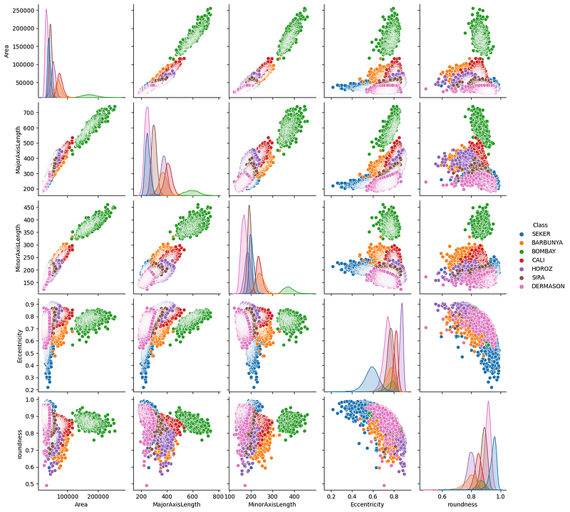
We see a few interesting trends — mainly, it seems that Bombay (green) beans are clearly separated from the others in terms of their physical measurements.

Let’s also plot a correlation matrix:

import matplotlib.pyplot as plt

correlation = beans.corr(numeric_only=True)

# Create a square heatmap with center at 0
sns.heatmap(correlation, center=0, square=True, cmap="coolwarm", vmin=-1, vmax=1)

plt.show()

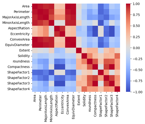
We have a few features almost perfectly correlated and that makes sense as they are related to physical measurements. However, we also have a few feature pairs that show no or very little correlation.

At this point, I will leave it to you to continue this exploration and try to find some questions to answer about the dataset.

Running an AutoML training job

To start an AutoML training job, we first need a dataset object compatible with it:

ds = ai.TabularDataset.create(
   display_name="dry_bean_dataset", gcs_source=gcs_path
)

TabularDataset created. 

type(ds)

google.cloud.aiplatform.datasets.tabular_dataset.TabularDataset

ds.resource_name

'projects/10783853768/locations/us-central1/datasets/4978116960081412096'

We use the TabularDataset.create method to initialize it as ds. Vertex AI assigns it its own name, which is accessible through its resource_name attribute.

Now, we initialize the job with ai.AutoMLTabularTrainingJob class. It requires two arguments:

• A display name for the job
• The objective of the task — classification, in this case.

job = ai.AutoMLTabularTrainingJob(
   display_name="dry-bean-classification",
   optimization_prediction_type="classification",
)

Next, we run the job’s run method:

model = job.run(
   dataset=ds,
   target_column="Class",
   training_fraction_split=0.8,
   validation_fraction_split=0.1,
   test_fraction_split=0.1,
   model_display_name="baseline-classification-model",
   disable_early_stopping=False,
)

The method’s parameters are fairly self-explanatory. The code will take some time to finish execution (depending on your compute power).

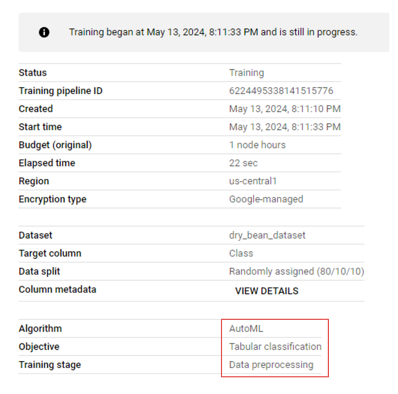
If you go to the “MODEL DEVELOPMENT > TRAINING” tab of your dashboard and click on the job name, you will see live training progress. The image below shows that the training is in the preprocessing stage:

Looking at results

Once training finishes, go to the training tab again and click on the model name. This time, there will be performance metrics listed alongside the model:

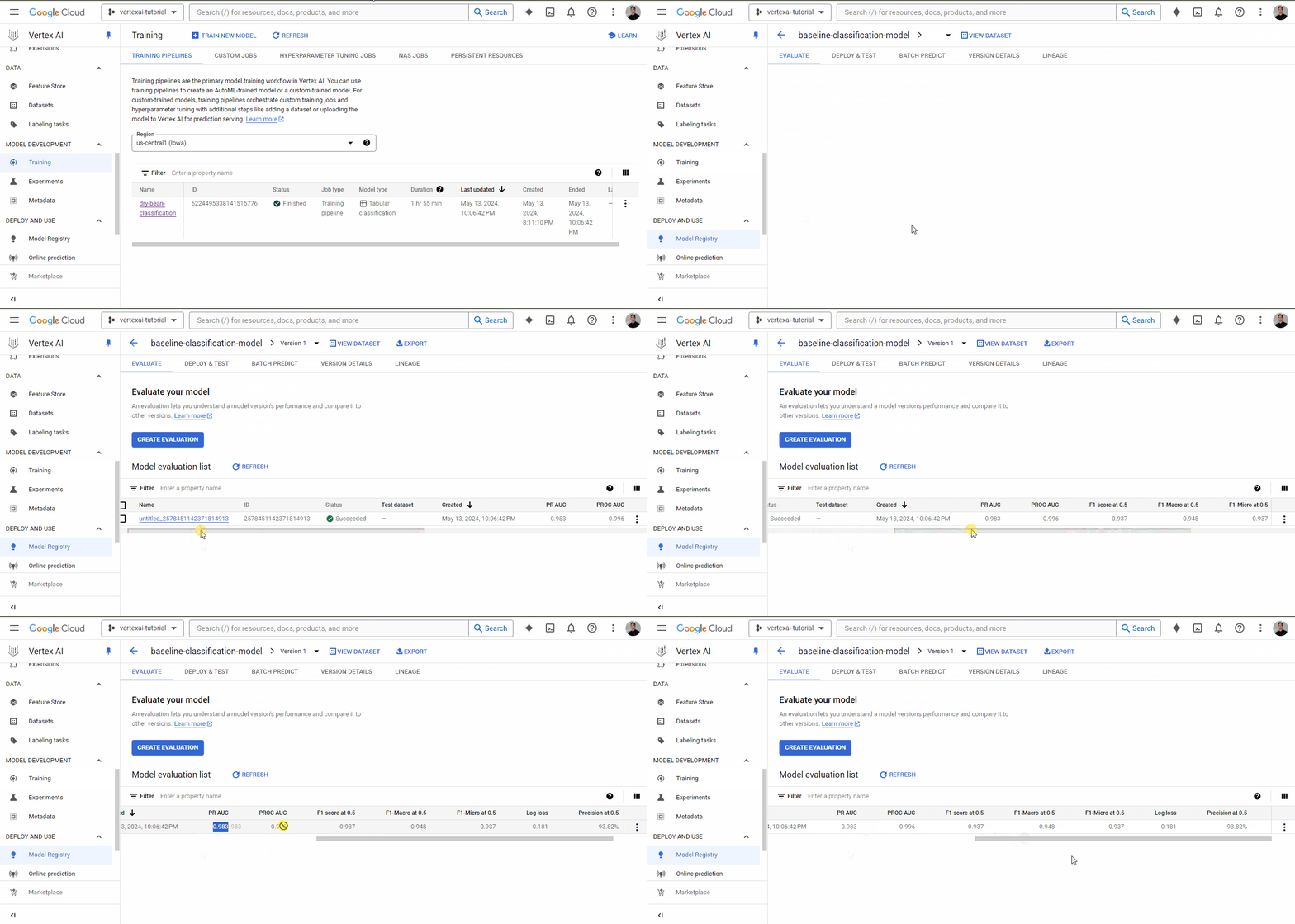
As you can see, even for a baseline model, we have very good metrics, all above 0.90.

Deploying an AutoML model and generating predictions

We can now deploy this model with a single line of code:

endpoint = model.deploy(machine_type="n1-standard-4")

The deploy method requires only a single argument - the type of machine to run inference. I won't actually run the above line as deploying incurs additional costs for as long as the model is online.

However, if you do run it, deploy method returns an Endpoint object we can send requests to:

prediction = endpoint.predict(
   [
       {
           "Area": "30099",
           "Perimeter": "638.8209999999999",
           "MajorAxisLength": "237.14191130827916",
           "MinorAxisLength": "162.3034300714102",
           "AspectRation": "1.4611022774068396",
           "Eccentricity": "0.7290928631259719",
           "ConvexArea": "30477",
           "EquivDiameter": "195.76321681302556",
           "Extent": "0.8036043251902283",
           "Solidity": "0.9875972044492568",
           "roundness": "0.9268374259664279",
           "Compactness": "0.8255108332939839",
           "ShapeFactor1": "0.007878730566074592",
           "ShapeFactor2": "0.002256976927384019",
           "ShapeFactor3": "0.6814681358857279",
           "ShapeFactor4": "0.9956946453228307",
       }
   ]
)

print(prediction)

It has a predict method that accepts a list of samples to predict. The samples must be given in JSON format.

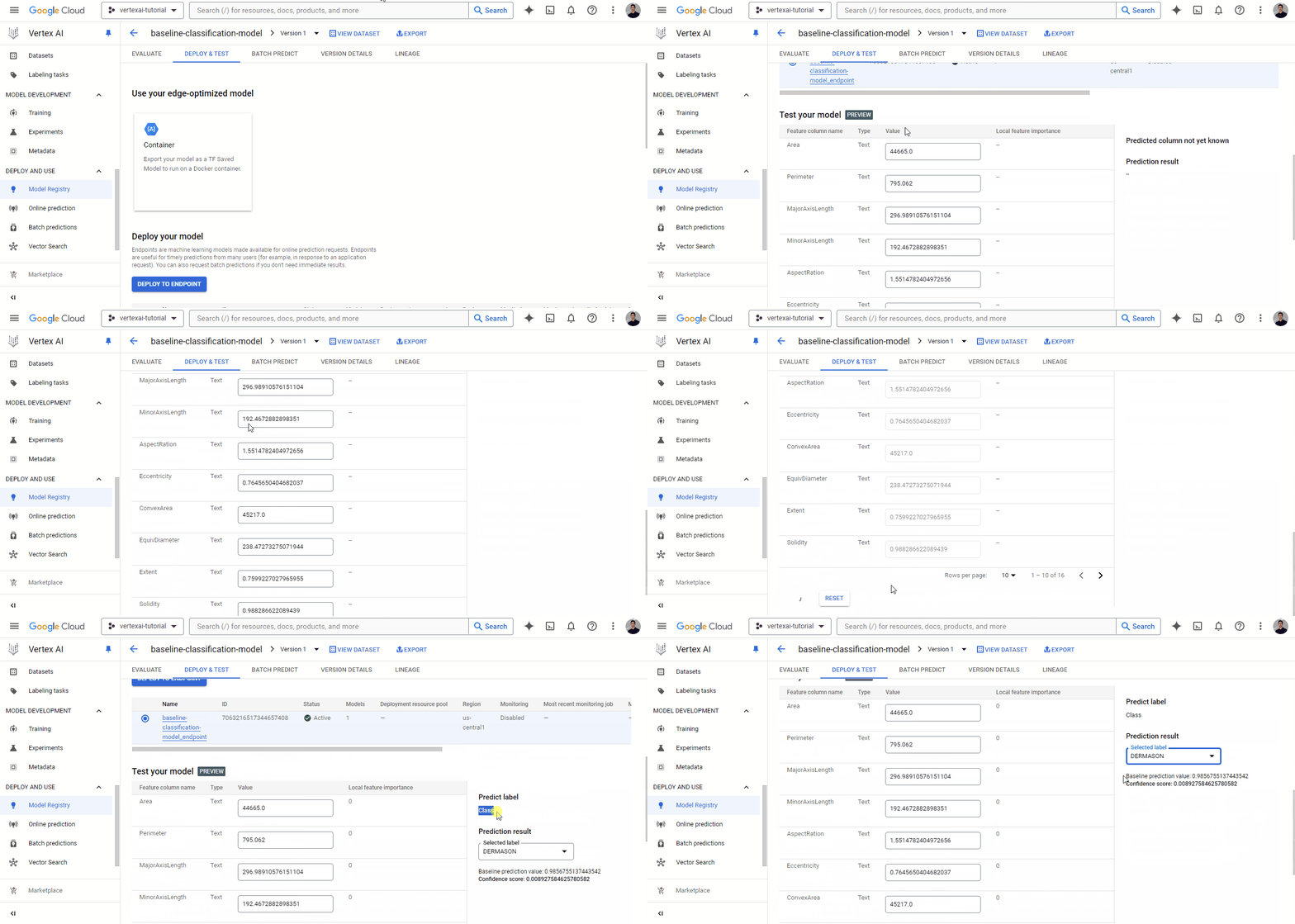
You can also use the dashboard to deploy models. If you go to the “MODEL REGISTRY” tab, you will see the model listed there. Click on its name and choose the “DEPLOY & TEST” tab:

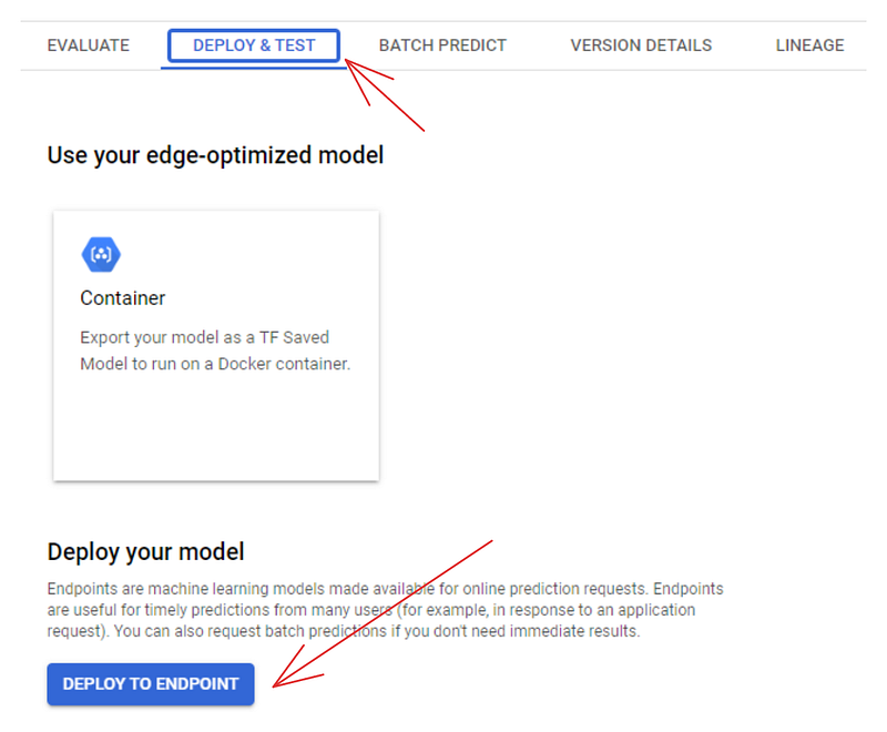
Clicking on the ‘DEPLOY TO ENDPOINT’ button takes you to a separate page where you can configure the machine to deploy your model. But before you do that, you can test it in the area below the deployment button:

Training and Deploying Custom Models in Vertex AI

Deploying custom models in Vertex AI is more challenging than AutoML models and also costs more because there will be some Docker containers involved on top of your Workbench and deployment expenses. If you are up for it, let’s go!

High-level overview of custom training in Vertex AI

Custom training involves starting with a custom model training script. In this script, we can do anything as long as it:

• Loads data from GCS bucket
• Trains a model with an ML framework (TF, PyTorch, Scikit-learn, XGBoost)
• Optionally, tunes the hyperparameters of the model
• Saves it to the GCS bucket to capture the trained or tuned model.

Then, this training script must be converted into a Docker container and then pushed to Google Container Registry. From there, we can use the Vertex AI Python SDK or the dashboard to train the custom model.

Creating a directory structure for the training code

First, let’s create the directory structure as recommended by this code lab by Google. In you workbench, switch to the terminal by starting a new launcher:

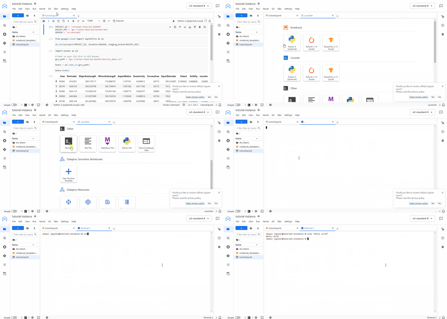
Then, create a new directory called “dry-beans” and change into it:

$ mkdir dry-beans
$ cd dry-beans/

Inside dry-beans, create another directory called trainer and inside it, train.py Python file:

$ mkdir trainer
$ touch trainer/train.py

Creating a Dockerfile

Next, create a new Dockerfile:

$ touch Dockerfile

Open the file and paste the following contents:

FROM gcr.io/deeplearning-platform-release/tf2-cpu.2-6
WORKDIR /

# Copies the trainer code to the docker image.
COPY trainer /trainer

# Install XGBoost
RUN pip install xgboost==1.6.2

# Sets up the entry point to invoke the trainer.
ENTRYPOINT ["python", "-m", "trainer.train"]

This Dockerfile uses the official deep learning image provided by Google Container Registry with TensorFlow installed. The file copies our trainer directory and then installs XGBoost. In the end, it will run our Python script.

Writing the training script

The script itself must load the Dry Beans dataset from our GCP bucket, train an XGBoost classifier on it and save the model back to the bucket. I’ve written a simple script that performs those tasks in this GitHub gist (I am not sharing it here to save space).

Copy/paste the code in the gist to train.py. Then, back in the terminal, install XGBoost since it doesn't come pre-installed in your chosen Workbench, and run the script:

$ pip install xgboost==1.6.2
$ python trainer/train.py

Building a Docker image

If the script runs without errors, continue by entering these two variables into the terminal:

$ PROJECT_ID='vertexai-tutorial-423010'  # Replace with your PROJECT_ID from earlier
$ IMAGE_URI="gcr.io/$PROJECT_ID/dry-beans:v1"  # This stays the same

These variables will be used when we build the container and so we do:

$ docker build ./ -t $IMAGE_URI

The build will take some time. After it finishes, run the container to make sure everything is running smoothly:

$ docker run $IMAGE_URI

Model trained successfully!
Model uploaded successfully!

If you get the success messages above, then the container is ready to push:

$ docker push $IMAGE_URI

Creating a custom training job

At this point, most of the battle is done. We can now switch to the dashboard and create a custom training job using the container we’ve just pushed. So, head over to the “MODEL REGISTRY” tab and click “CREATE”:

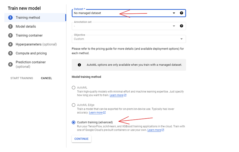
For the training method, choose the “No managed dataset” and “Custom training” options. In the next pane (Model details), give the model a name — dry-beans-classifier.

In the training container pane:

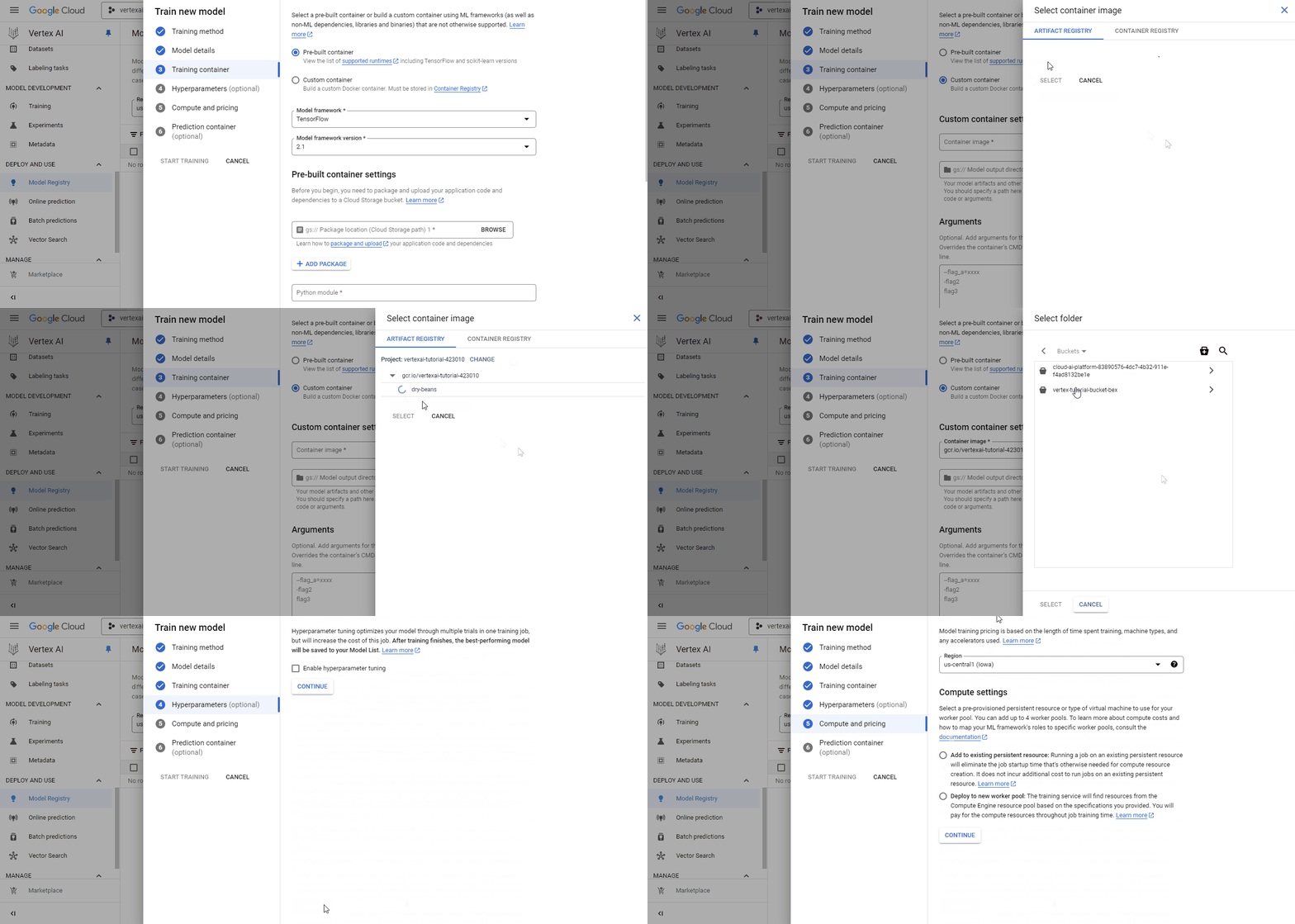
Select the container we’ve pushed for the custom image and the cloud-ai-platform bucket for model output. Then, click continue until you reach the "Compute and pricing" pane:

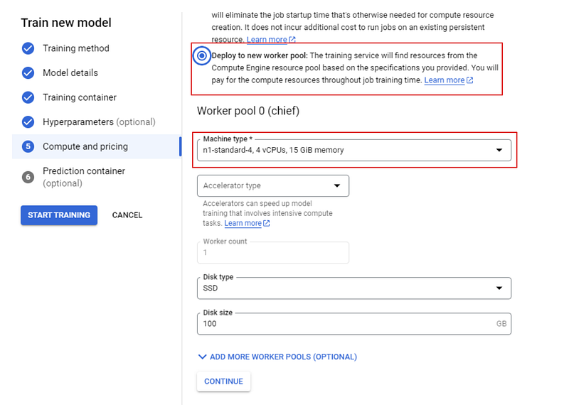
Choose a standard n1 machine with 4 CPUs and finally, click "START TRAINING". Then, switch to the "TRAINING" tab of your dashboard.

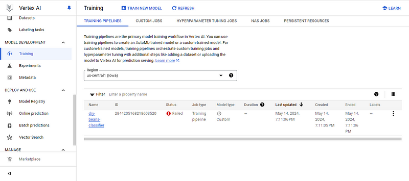
At this point, you will see one of two things:

1. The training failed status
2. The training in progress status

I have the former one, so let’s investigate why by clicking on the model name:

The error is telling me that I exceeded the number of allowed custom training CPUs. I’ve dug deeper into the issue and what I found was very disappointing.

Normally, GCP gives at least 20 CPU quotas for any compute region, but after checking my profile, I discovered that my quota was only 1. This meant that I couldn’t run any custom training jobs, as all machines offered by Google have at least two CPUs.

I tried to increase my quota using the answers from this StackOverflow thread, but they didn’t work. The message I got was that new Vertex AI users were only allowed a single CPU unit. If I wanted to increase my quota, I would need to submit a support ticket, which, as it turns out, isn’t free (you need a paid support contract).

So, if you are unlucky like me, try the answers in the SO thread. They worked for some people, but if they don’t work for you, then your only option is to contact support.

But if you are lucky and your training finishes, then you will be able to deploy the model using the same steps I outlined for AutoML models.

Conclusion

Vertex AI is a massive platform with many features. In this tutorial, we have barely scratched the surface but we’ve covered the most important building blocks of the platform. By mastering the creation of storage buckets, workbenches, and training jobs, you will be well-equipped to explore the rest of the platform.

If you want to learn more about Google Cloud services, check out these recommended related resources:

• Introduction to GCP course
• Google Cloud For Data Science Tutorial
• AWS vs. Azure vs. GCP Services Comparison
• Google Gemini Tutorial