XMATCH in Excel Tutorial: Overview, Syntax, and Practical Applications

There are many situations during your data analyses where you will need to find the relative position of an item in an array or range of cells given a certain value or pattern. 

The most effective way to conduct pattern-matching operations in Excel is the XMATCH function. A simple yet powerful function, XMATCH has several features that enable precise and flexible matching. 

In this tutorial, we will cover the basics of the Excel XMATCH function, analyze its syntax and different parameters, and provide practical examples to illustrate its capabilities. We will also compare XMATCH with MATCH, another popular function used for similar tasks.  Finally, we will look at common pitfalls when using the XMATCH function and lay down best practices to ensure sound and efficient use.

If you’re on your Excel learning journey and want to find out more, check out our Excel Fundamentals skill track to learn all the essentials. 

What is XMATCH?

XMATCH is a flexible and robust function for matching operations. XMATCH() allows you to perform all kinds of matching operations, from vertical and horizontal look-ups to exact, approximate, and partial matches. 

For those who have been using Excel for a long time, you will probably be familiar with the MATCH function. Before the Excel update introducing XMATCH, MATCH was the go-to function for matching tasks. You can learn about these in our Excel Lookup Functions tutorial. 

However, as we will see later, MATCH can fall short in certain scenarios. In this regard, XMATCH can be seen as an improved and long-awaited upgrade of the traditional MATCH function, providing search in any direction and multiple match types, making it easier and suitable for a wider range of use cases.

Note that the function is only available in Excel for Microsoft 365 and Excel 2021. For users with previous versions of Excel, MATCH is still the only available function.

Let’s now have a look at the XMATCH syntax and parameters. 

XMATCH Syntax and Parameters

Here is the basic syntax of the XMATCH function:

=XMATCH(lookup_value, lookup_array, [match_mode], [search_mode])

The function comes with two required arguments (i.e., lookup_value and lookup_array) and two optional ones (match_mode and search_mode) that provide capabilities for more precise and flexible operations.

Below, you can find a description of the four parameters:

• Lookup_value: It’s the value to look for.
• Lookup_array: It’s the array or list where to search. It can be a vertical or a horizontal lookup array.
• Match_mode: allows you to choose the match type. There are four modes, including:
• 0: Exact match (the default mode)
• -1: Exact match or next smallest item
• 1: Exact match or next largest item
• 2: A wildcard match, such as * and ?.
• Search_mode: allows you to specify the search mode, including the search direction and algorithm. There are four possible values:
• 1: Search first-to-last (the default value)
• -1: Search last-to-first (reverse search).
• 2:  Binary search ascending. The search is performed assuming the lookup array is sorted in ascending order, otherwise, it returns invalid results.
• -2:  Binary search descending. The search is performed assuming the lookup array is sorted in descending order, otherwise, it returns invalid results.

Match Modes: Precision and Flexibility

XMATCH comes with an optional match_mode parameter that allows you to choose the match type. These options come in very handy, providing ways to conduct both precise matching and approximate matching. Let’s analyze in detail the available match modes:

Exact match

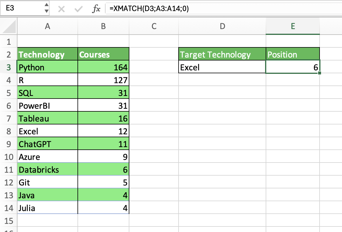
Exact match (match_mode = 0) is the default match mode of XMATCH. It means that Excel will find an exact match of the lookup value in the lookup array, otherwise, it will return a NA error. Exactly matching is essential when accuracy and precision are key, such as finding specific entries in a database.

Here is a basic example on how to use the XMATCH function to find the exact position of “Excel” in a list of technologies available in the DataCamp Course Catalog. We provide the lookup value in D3 and the lookup array (A3:A14), and Excel correctly gives the position 6. 

Approximate match

There may be situations where you need to make a flexible match, either because you don’t know the exact lookup value or because you’re looking for approximate results. 

Fortunately, XMATCH comes with two match modes that allow you to perform exact or next-smallest and exact or next-largest values. 

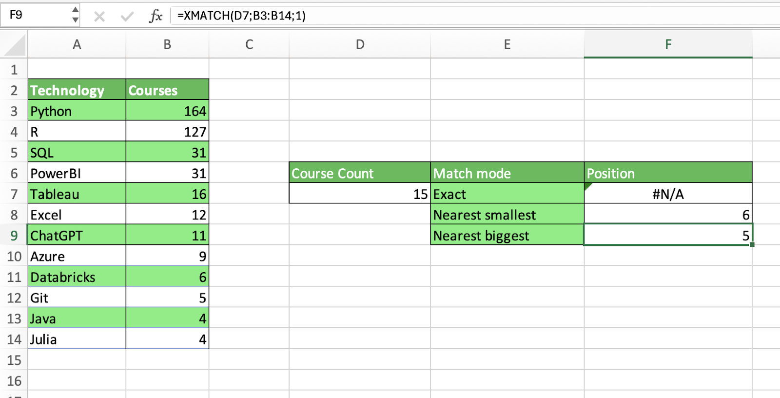
In the following example, we use approximate matching to find the closest counts of courses to the lookup value 15. 

When using the next smallest (match_mode = -1), Excel returns the position 6, for 12 courses is the nearest smallest number in the list. In the case of the next biggest, Excel returns 5, for 16 courses is the nearest biggest number.

We also use the exact match to illustrate what happens when Excel cannot find an exact match.

Wildcard and regex matches

An innovative feature in XMATCH is the possibility to use basic wildcards when you set match_mode to 2, as well as more advanced regular expressions if set to 3. These match modes only work with text data.

XMATCH allows you to use two popular wildcards:

• ?: to match any single character.
• *: to match any sequence of characters.

Below, you can find various examples of how to use regex matches. In the first example, we look for technologies that start with an E. Second, we look for technologies with an A in their name. Finally, we look for technologies with three letters.

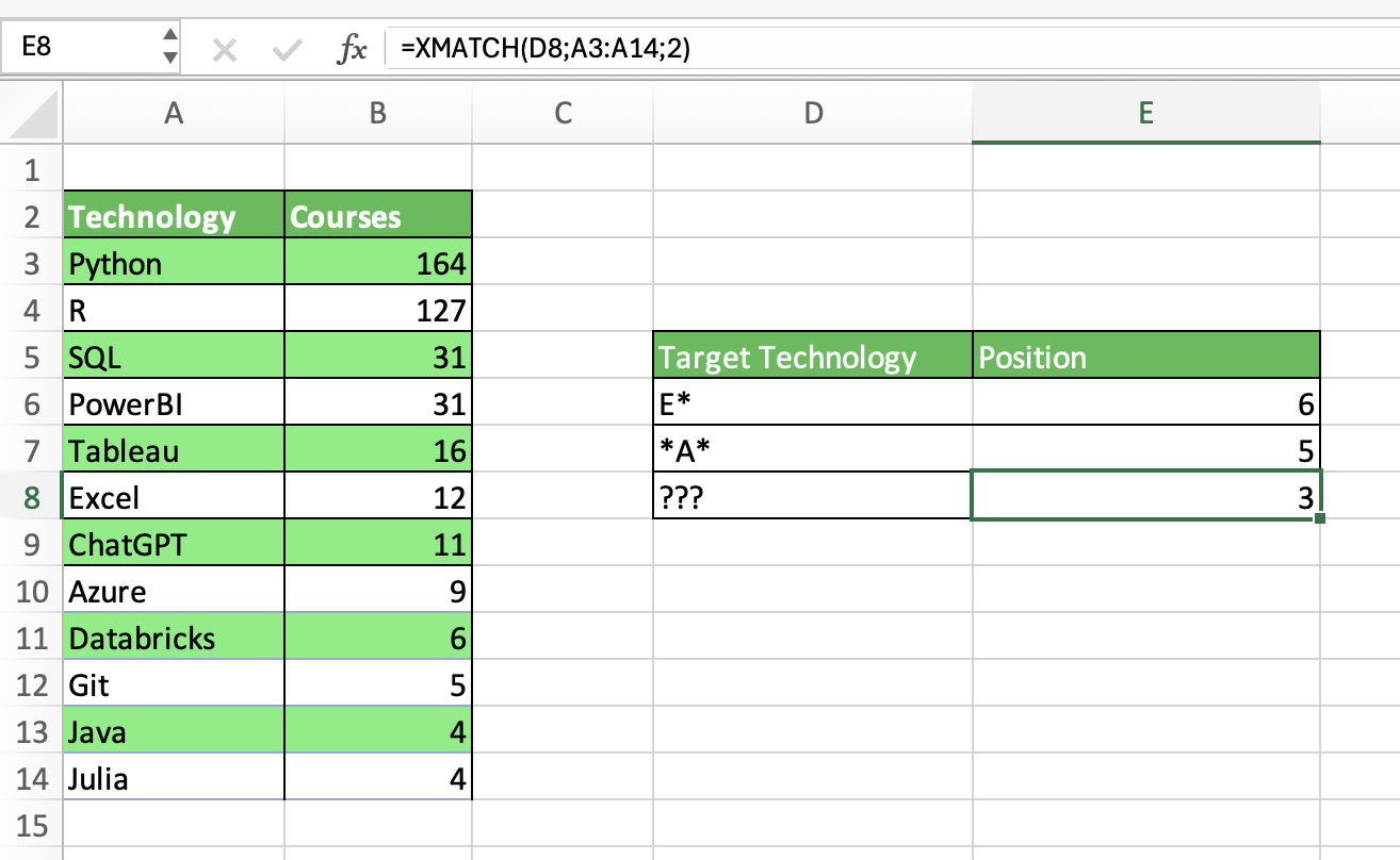
Notice that XMATCH will always return the first occurrence in the lookup array, unless we specify differently (see next section).

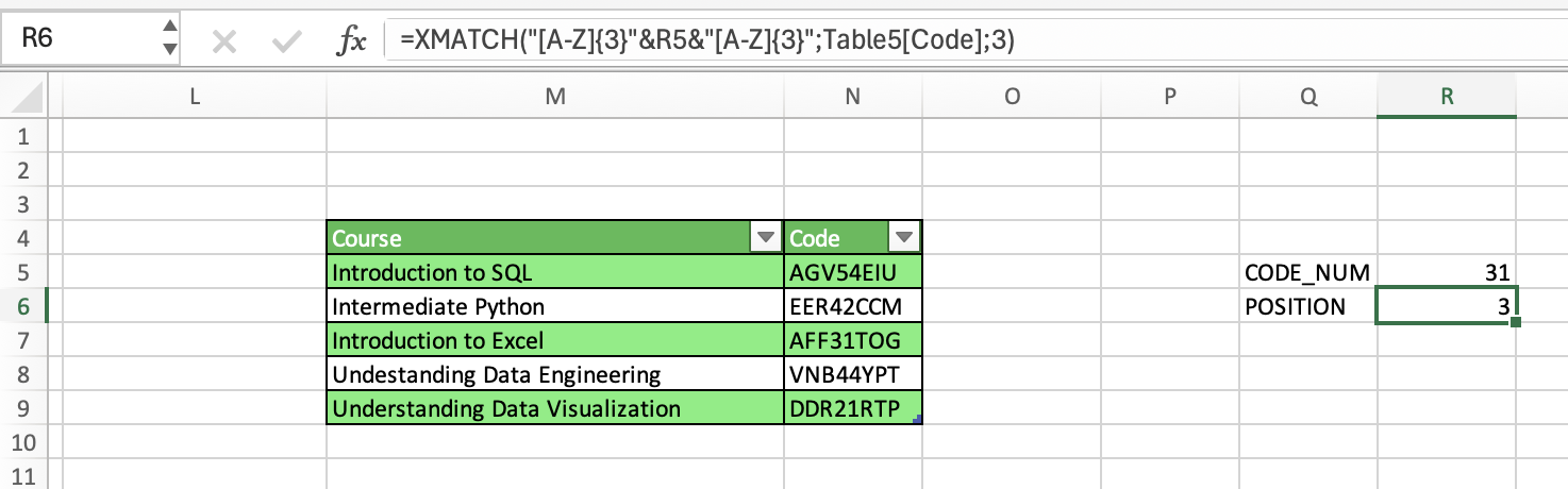
If you want to use more complex regular expressions, turn match_mode to 3. Regular expressions, often abbreviated as "regex" or "regexp," are a way to define a search pattern, which can be used for various text manipulation tasks such as searching, parsing, and/or replacing text. 

For more details about pattern matching, our Excel Regex Tutorial: Mastering Pattern Matching with Regular Expressions is a great place to get started.

Here is a rather simple example: We want to find the position of a course whose code includes three letters at the beginning, three at the end, and two numbers in the middle (31).

XMATCH Search Modes: Direction and Efficiency

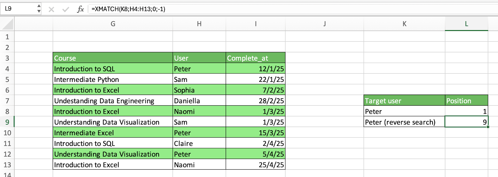
XMATCH introduces a new parameter that allows you to control the direction of the search. This feature is great when you’re more interested in finding the last occurrence rather than the first, for example, for certain tasks in time series analysis. 

Let’s explore in detail the different search modes.

Reverse search

To perform a reverse search, you can set the search_mode parameter to -1. For example, below you can see how to find the first and the last course completed by the user Peter.

Binary search

Finally, the search_mode parameter also comes with the possibility to use a binary search algorithm to conduct the matching operation. Binary search is a sorting algorithm that works by repeatedly dividing the search interval in half. It’s one of the most effective sorting algorithms, but it requires the input data to be previously sorted. 

XMATCH allows you to leverage binary search given an array sorted in both ascending (search_mode = 2) and descending (search_mode = -2). In case the lookup array is not sorted, the function will throw an error.

Practical Applications and Examples of XMATCH

XMATCH is well-suited for a wide array of Excel tasks, from basic to advanced. In this section, we cover some of the most compelling practical applications.

Two-dimensional lookups with INDEX/XMATCH

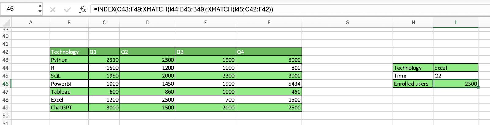
The INDEX and XMATCH functions can work in tandem to conduct two-dimensional lookups, that is, looking up in rows and columns simultaneously. By combining these two functions, we can create a dynamic lookup that works great in domains, such as a financial analysis, where is very common to compare variables across categories. 

For example, in the image below, we combine INDEX and MATCH to extract the number of enrolled users in Excel courses during Q2. INDEX takes three arguments here: the array where to find the value, the row number, and the column number. The values of the last two arguments are provided by multiple XMATCH functions.

 If we would like to change the technology at hand or the Quarter, you just have to change the lookup values in the XMATCH functions, and the result of the INDEX will change along the way.

The INDEX/XMATCH works in a very similar fashion to INDEX/MATCH. If you want to know about this powerful tandem with practical examples, check out our how to INDEX MATCH Multiple Criteria in Excel Tutorial.

Multi-column lookups

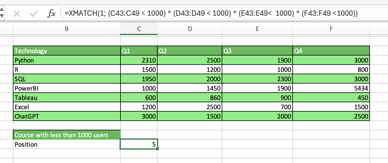
Another great use of XMATCH is to combine multiple criteria to create multi-column lookups. This may not seem intuitive, as XMATCH look requires a lookup value and a lookup array to work. But we can use Boolean logic to create a temporary array within the XMATCH formula that contains zeros and ones to represent rows matching the criteria you specify. 

For example, say you want to find the first technology in the list that has fewer than 1000 enrolled users every quarter. You can combine the conditions by combining the results in every column using the * symbol. Excel will find under the hood the array containing all ones, in our case, Tableau, hence the position 5.

Dynamic array filtering

XMATCH can also work hand in hand with the FILTER and ISNUMBER functions to enhance dynamic array filtering.

Below, you can find out how it works. We will use these functions to filter the information of completed courses by users based on the user name. 

First, we use  XMATCH to calculate the relative position of every user in the table based on the lookup array with the names we will use to filter. This will give us a table with the relative position of every name, including null values for users not included in the filter list.

Then, we convert the column with relative positions and null values to TRUE or FALSE using the ISNUMBER function.

Finally, we use FILTER to select all the columns we want to display, and the column with TRUE and FALSE to filter rows.

Addressing null values with ISNA

When XMATCH cannot find any match, it will return an NA error. While this is already informative, you can prettify the results and prevent misinterpretations by using the ISNA and IF functions.

Imagine we have a table with the courses completed by Sam and Peter, and we want to know which courses they have in common. If we just use XMATCH, Excel will return the relative position of common courses, and null values otherwise. If we pass XMATCH as the argument of ISNA, the function will return TRUE or FALSE instead. Then, by using the IF function, we can change the boolean values for other messages.

Binary search for large datasets

We already mentioned that XMATCH allows you to use a binary search algorithm during matching operations. This feature can be a game-changer when dealing with large datasets. Provided that the lookup array is sorted, opting for the binary search engine can speed up your matching operations dramatically.

XMATCH vs MATCH: Key Differences

As already mentioned, XMATCH was designed to supersede the traditional MATCH function. Both have the same purpose, but XMATCH comes with a set of new capabilities, making it more powerful than MATCH. Below, you can find a list of the main differences between XMATCH vs MATCH:

Common Pitfalls and Solutions

There are many potential uses of XMATCH. However, it’s important to mention common problems you may encounter while using it. Here is a list of some regular pitfalls and tips to address them.

• Check data types: XMATCH will have an unexpected behaviour if you apply it to a range with the wrong data type. Hence, before applying the function, make sure you have set the right data types for your columns.
• Range consistency: While XMATCH allows for horizontal and vertical lookup ranges, mixing them can lead to unexpected problems and performance issues. When possible, try to be consistent and choose either horizontal or vertical ranges.
• Leverage match modes: XMATCH comes with various match modes. The default mode is exact match, but you can also fine-tune your lookups by using approximate searches and regex operations.
• Better with sorted arrays: Overall, the performance of XMATCH will always be higher if you apply it to sorted arrays. This is true for the default function, and a mandatory prerequisite if you want to use binary search. 
• Handling N/A errors:  As already mentioned, XMATCH will throw an NA error if there is no match in your lookups. The best way to address this and enhance readability is by passing the results to a combination of IF AND ISNA functions, or to an IFNA function.

Performance Considerations

XMATCH is not the only function to perform lookup operations in Excel. For example, you may consider using VLOOKUP, HLOOKUP, or even legacy functions like MATCH. However, when it comes to search speed, XMATCH is arguably the fastest, especially if you apply it to ordered arrays, where you can also leverage the power of binary search.

It’s also worth mentioning that XMATCH is designed as a dynamic array formula, meaning that it can return arrays of variable size depending on the input data. Dynamic array formulas are especially well-suited when working with large datasets or complex calculations. 

Conclusion

Congratulations on making it to the end. XMATCH is a powerful function, and you cannot miss it in your Excel data analyses. Either as a standalone function or in tandem with other Excel functions, XMATCH will take your lookup operations to a new level. 

But there is much more to know in the wonderful world of Excel. Check out our dedicated courses, blogs, and tutorials to become an Excel wizard:

• XLOOKUP() vs. VLOOKUP(): A Comparison for Excel Users
• Data Manipulation in Excel Cheat Sheet 
• Excel | Master Advanced Techniques Course
• Intermediate Power Query in Excel 
• Excel Shortcuts Cheat Sheet 
• Excel Formulas Cheat Sheet 
• How to INDEX MATCH Multiple Criteria in Excel 
• Data Wrangling with INDEX-MATCH in Spreadsheets 
• Excel Regex Tutorial: Mastering Pattern Matching with Regular Expressions