

What Is PySpark?
PySpark is the Python API for Apache Spark. Your Python code describes the transformations you want, and Spark's engine, which runs on the Java Virtual Machine (JVM), plans and executes them across the cluster. You get Spark's distributed execution without writing Scala or Java.
Data scientists use PySpark to clean and aggregate large datasets, data engineers use it for ETL pipelines, and both use pyspark.ml to train models on data that won't fit on one machine. If most of your work happens in pandas today, the DataFrame API will feel familiar.
When to use PySpark instead of pandas
PySpark pays off when data outgrows a single machine; below that, pandas is usually faster because it has no JVM startup or task scheduling overhead.
| Feature | pandas | PySpark |
|---|---|---|
| Data size | Limited by one machine's RAM | Limited by the cluster's combined memory and disk |
| Execution | Eager, mostly single core | Lazy, parallel across cores or machines |
| Startup overhead | None | A few seconds to start the JVM and SparkSession |
| Streaming data | Not supported | Structured Streaming |
| Machine learning | scikit-learn ecosystem | pyspark.ml (distributed) |
| Fault tolerance | None; a crash loses the work | Lost partitions are recomputed from their lineage |
My rule of thumb: if the data fits in memory with room to spare and the job runs on one laptop, stay with pandas. Switch to PySpark when you're fighting memory errors, or when the job will eventually run on a cluster or a platform like Databricks.
How to Install PySpark
PySpark installs from PyPI with one pip command, which bundles the Spark runtime, so you don't need a separate Spark or Hadoop download for local work. Before running it, check the two prerequisites.
Prerequisites
According to the official installation guide, PySpark 4.3 requires:
- Python 3.11 or later. PySpark 4.3 dropped Python 3.10; see our Python setup guide if you need a newer version.
- Java 17 or later (Spark 4.3 runs on Java 17, 21, and 25) with the
JAVA_HOMEenvironment variable pointing to it. Our guide to installing Java walks through each operating system.
You can check both from a terminal:
python3 --version # Python 3.11 or later
java -version # openjdk version "17" or laterIf you work in DataLab or Databricks, PySpark is already installed, and you can skip to the dataset.
Installing PySpark with pip
I recommend a virtual environment so PySpark's dependencies don't collide with other projects:
python3 -m venv pyspark-env
source pyspark-env/bin/activate
pip install "pyspark[sql]" "pandas<3"
python3 -c "import pyspark; print(pyspark.__version__)"4.3.0On Windows, use python instead of python3, and activate the environment with pyspark-env\Scripts\activate. The [sql] extra adds pandas, PyArrow, and NumPy, which PySpark uses for toPandas() and pandas UDFs. I pin pandas<3 because PySpark 4.3 prints a warning that it doesn't yet fully support pandas 3.0.
Two errors account for most failed first runs:
JAVA_GATEWAY_EXITEDor "Unable to locate a Java Runtime": Java is missing orJAVA_HOMEisn't set.PYTHON_VERSION_MISMATCH: Spark's worker processes picked up a different Python than your script. SetPYSPARK_PYTHONto your environment's interpreter, for exampleexport PYSPARK_PYTHON=$(which python).
For operating-system-specific steps, including Windows, see our PySpark installation guide.
Getting the dataset
The examples use an e-commerce dataset of 541,909 transactions from a UK-based online retailer, covering December 2010 to December 2011. Each row is one product line on an invoice, with 8 columns:
InvoiceNo: invoice number (numbers starting with "C" are cancellations)StockCodeandDescription: product code and nameQuantityandUnitPrice: units bought and price per unit, in pounds sterlingInvoiceDate: date and time of the purchaseCustomerID: customer identifier (missing on some rows)Country: the customer's country
You can download it as datacamp_ecommerce.csv from the DataLab dataset page. It's the Online Retail dataset from the UCI Machine Learning Repository, so you can also build the same file from the public source (requires pip install openpyxl):
import io
import urllib.request
import zipfile
import pandas as pd
url = "https://archive.ics.uci.edu/static/public/352/online+retail.zip"
with urllib.request.urlopen(url) as response:
archive = zipfile.ZipFile(io.BytesIO(response.read()))
retail = pd.read_excel(
archive.open("Online Retail.xlsx"),
dtype={"InvoiceNo": str, "StockCode": str, "CustomerID": "Int64"},
)
# Match the DataLab file's date format, e.g. 12/1/10 8:26
retail["InvoiceDate"] = retail["InvoiceDate"].map(
lambda ts: f"{ts.month}/{ts.day}/{ts:%y} {ts.hour}:{ts:%M}"
)
retail.to_csv("datacamp_ecommerce.csv", index=False)Reading the 23 MB Excel file takes about a minute. Save the CSV in the folder you'll run the rest of the code from.
Creating a SparkSession
A SparkSession is the entry point to every PySpark program: it connects your Python code to the Spark engine and creates DataFrames. You create one per application with the builder pattern:
from pyspark.sql import SparkSession
spark = SparkSession.builder.appName("PySparkTutorial").getOrCreate()
print(spark.version)4.3.0getOrCreate() returns the running session if one exists, so it's safe to call twice in a notebook. Launched from a plain Python process, Spark runs in local mode (local[*]), using every CPU core on your machine as a worker, and serves the Spark UI at http://localhost:4040 for watching jobs. When you're done, spark.stop() releases the resources.
Loading the e-commerce dataset
With the session running, we can read the CSV into a DataFrame. I pass an explicit schema rather than inferSchema=True, which makes Spark scan the whole file an extra time just to guess column types:
import pyspark.sql.functions as F
schema = """
InvoiceNo STRING, StockCode STRING, Description STRING, Quantity INT,
InvoiceDate STRING, UnitPrice DOUBLE, CustomerID INT, Country STRING
"""
orders = spark.read.csv(
"datacamp_ecommerce.csv", header=True, schema=schema, escape='"'
)
orders = orders.withColumn("InvoiceDate", F.to_timestamp("InvoiceDate", "M/d/yy H:mm"))
orders.printSchema()root
|-- InvoiceNo: string (nullable = true)
|-- StockCode: string (nullable = true)
|-- Description: string (nullable = true)
|-- Quantity: integer (nullable = true)
|-- InvoiceDate: timestamp (nullable = true)
|-- UnitPrice: double (nullable = true)
|-- CustomerID: integer (nullable = true)
|-- Country: string (nullable = true)Two details in that snippet matter:
escape='"'handles product names that contain doubled quotes, such asRECORD FRAME 7"" SINGLE SIZE. Spark's default escape character is a backslash.- The date pattern
M/d/yy H:mmmatches values like12/1/10 8:26. Since Spark 4.0, ANSI SQL mode is on by default, soto_timestamp()raises aCANNOT_PARSE_TIMESTAMPerror on a value that doesn't match the pattern. UseF.try_to_timestamp()if you'd rather getNULLfor bad rows.
To look at the first rows and count them:
orders.show(5, truncate=False)
print(orders.count())+---------+---------+-----------------------------------+--------+-------------------+---------+----------+--------------+
|InvoiceNo|StockCode|Description |Quantity|InvoiceDate |UnitPrice|CustomerID|Country |
+---------+---------+-----------------------------------+--------+-------------------+---------+----------+--------------+
|536365 |85123A |WHITE HANGING HEART T-LIGHT HOLDER |6 |2010-12-01 08:26:00|2.55 |17850 |United Kingdom|
|536365 |71053 |WHITE METAL LANTERN |6 |2010-12-01 08:26:00|3.39 |17850 |United Kingdom|
|536365 |84406B |CREAM CUPID HEARTS COAT HANGER |8 |2010-12-01 08:26:00|2.75 |17850 |United Kingdom|
|536365 |84029G |KNITTED UNION FLAG HOT WATER BOTTLE|6 |2010-12-01 08:26:00|3.39 |17850 |United Kingdom|
|536365 |84029E |RED WOOLLY HOTTIE WHITE HEART. |6 |2010-12-01 08:26:00|3.39 |17850 |United Kingdom|
+---------+---------+-----------------------------------+--------+-------------------+---------+----------+--------------+
only showing top 5 rows
541909For more reading options, such as multiple files, delimiters, and corrupt records, see our PySpark read CSV tutorial.
RDDs vs. DataFrames
RDDs and DataFrames are PySpark's two ways to represent distributed data, and for almost all new code, DataFrames are the right choice.
| Abstraction | What it is | When to use it |
|---|---|---|
| RDD (Resilient Distributed Dataset) | Low-level, immutable collection of arbitrary Python objects, split into partitions | Unstructured data, or when you need fine-grained control over partitioning |
| DataFrame | Distributed table with named, typed columns, similar to a pandas DataFrame | Analysis, SQL queries, ETL, and machine learning |
Here's the same aggregation, total quantity per country, written both ways:
sales = [("United Kingdom", 6), ("France", 24), ("United Kingdom", 8)]
# RDD: you write the logic with Python functions
rdd = spark.sparkContext.parallelize(sales)
print(rdd.reduceByKey(lambda a, b: a + b).collect())
# DataFrame: you declare the result, and Spark plans how to compute it
sales_df = spark.createDataFrame(sales, ["country", "quantity"])
sales_df.groupBy("country").sum("quantity").show()[('France', 24), ('United Kingdom', 14)]
+--------------+-------------+
| country|sum(quantity)|
+--------------+-------------+
|United Kingdom| 14|
| France| 24|
+--------------+-------------+The RDD version runs your lambda in Python worker processes. The DataFrame version goes through Spark's Catalyst optimizer, which rewrites the query into an efficient plan that runs inside the JVM, so DataFrame code is usually faster without any tuning. The rest of this tutorial uses DataFrames.
Lazy Evaluation: Transformations vs. Actions
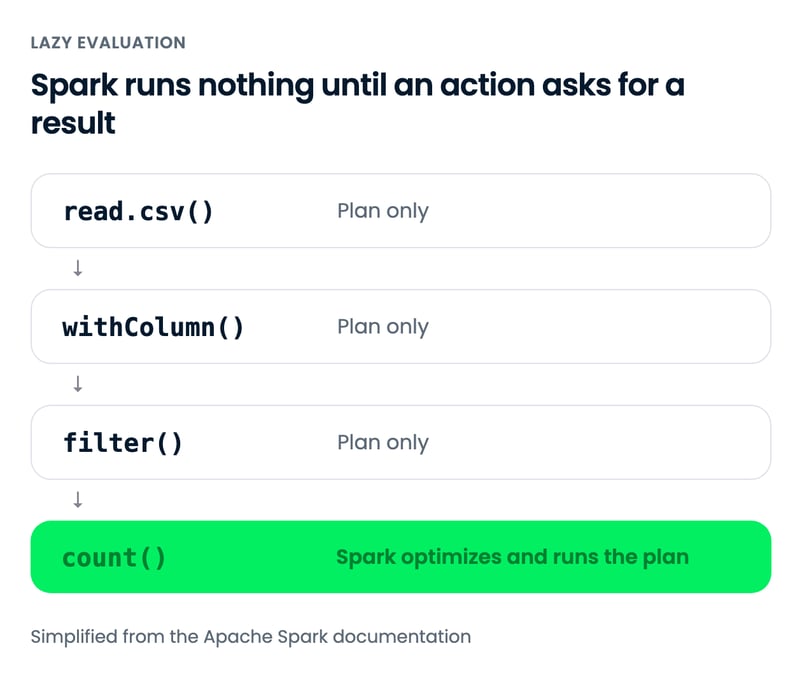
Lazy evaluation means Spark doesn't execute a transformation when you call it; it records the step in a plan and runs the whole plan only when an action asks for a result.
| Transformations | Actions | |
|---|---|---|
| What they do | Describe a new DataFrame | Return a result or write data |
| When they run | Never on their own | Immediately, triggering every pending transformation |
| Examples | select(), filter(), withColumn(), groupBy(), join() | show(), count(), collect(), toPandas(), write |
The filter below returns instantly, even though the dataset has over half a million rows, because nothing is read yet. The count() call is what launches a job:
uk_orders = orders.filter(F.col("Country") == "United Kingdom") # transformation: no job yet
print(uk_orders.count()) # action: Spark reads the file now495478Waiting until an action lets Spark optimize the whole chain at once. explain() prints the physical plan it chose (trimmed here):
uk_orders.explain()== Physical Plan ==
*(1) Project [InvoiceNo#0, StockCode#1, ...]
+- *(1) Filter (isnotnull(Country#7) AND (Country#7 = United Kingdom))
+- FileScan csv [...] PushedFilters: [IsNotNull(Country), EqualTo(Country,United Kingdom)], ...The PushedFilters entry shows Spark pushing the country filter down into the file scan, so rows from other countries are dropped as the CSV is read. One practical consequence: a data error inside a transformation, such as a date that fails to parse under ANSI mode, surfaces only when the next action runs, several lines later.
Common DataFrame Operations
Most PySpark code is a chain of five DataFrame operations: select(), filter(), withColumn(), groupBy(), and join(). Each returns a new DataFrame, so you can chain them in any order.
Selecting columns with select()
select() returns a DataFrame with only the columns you name:
orders.select("InvoiceNo", "Description", "Quantity", "UnitPrice").show(3, truncate=False)+---------+----------------------------------+--------+---------+
|InvoiceNo|Description |Quantity|UnitPrice|
+---------+----------------------------------+--------+---------+
|536365 |WHITE HANGING HEART T-LIGHT HOLDER|6 |2.55 |
|536365 |WHITE METAL LANTERN |6 |3.39 |
|536365 |CREAM CUPID HEARTS COAT HANGER |8 |2.75 |
+---------+----------------------------------+--------+---------+
only showing top 3 rowsFiltering rows with filter()
filter() keeps the rows that match a condition. This dataset mixes sales with cancellations (invoice numbers starting with "C"), negative quantities, and rows without a customer, so I'll keep only valid sales:
sales_only = orders.filter(
(F.col("Quantity") > 0)
& (F.col("UnitPrice") > 0)
& F.col("CustomerID").isNotNull()
& ~F.col("InvoiceNo").startswith("C")
)
print(sales_only.count())397884Combine conditions with & (and), | (or), and ~ (not), and wrap each one in parentheses, because Python's operator precedence would otherwise evaluate & before >. Our PySpark filter tutorial covers more patterns.
Adding columns with withColumn()
withColumn() adds a column, or replaces one with the same name. Here it calculates the value of each line:
sales_only = sales_only.withColumn("TotalAmount", F.round(F.col("Quantity") * F.col("UnitPrice"), 2))
sales_only.select("InvoiceNo", "Quantity", "UnitPrice", "TotalAmount").show(3)+---------+--------+---------+-----------+
|InvoiceNo|Quantity|UnitPrice|TotalAmount|
+---------+--------+---------+-----------+
| 536365| 6| 2.55| 15.3|
| 536365| 6| 3.39| 20.34|
| 536365| 8| 2.75| 22.0|
+---------+--------+---------+-----------+
only showing top 3 rowsSee our PySpark withColumn() tutorial for conditional columns with F.when().
Aggregating with groupBy() and agg()
groupBy() groups rows by one or more columns, and agg() computes one or more summaries per group. Which countries bring in the most revenue?
country_revenue = (
sales_only.groupBy("Country")
.agg(
F.count_distinct("CustomerID").alias("customers"),
F.round(F.sum("TotalAmount"), 2).alias("revenue"),
)
.orderBy(F.desc("revenue"))
)
country_revenue.show(5)+--------------+---------+----------+
| Country|customers| revenue|
+--------------+---------+----------+
|United Kingdom| 3920|7308391.55|
| Netherlands| 9| 285446.34|
| EIRE| 3| 265545.9|
| Germany| 94| 228867.14|
| France| 87| 209024.05|
+--------------+---------+----------+
only showing top 5 rowsThe UK dominates, as you'd expect from a UK retailer. The more interesting rows are the Netherlands and Ireland (listed as EIRE): 9 and 3 customers spend more than Germany's 94, which suggests wholesale buyers.
Notice I import the functions module as F instead of using from pyspark.sql.functions import *, which shadows Python's built-in sum(), min(), and max(). Since PySpark 4.0, that wildcard import also no longer exposes the old camelCase name countDistinct.
Our PySpark groupBy tutorial goes deeper into aggregations.
Joining DataFrames with join()
join() combines two DataFrames on a shared key. To label each country with a region, I'll join a small lookup table that deliberately leaves out Australia:
regions = spark.createDataFrame(
[("United Kingdom", "UK"), ("Netherlands", "EU"), ("EIRE", "EU"),
("Germany", "EU"), ("France", "EU")],
["Country", "region"],
)
country_revenue.join(regions, on="Country", how="left").orderBy(F.desc("revenue")).show(6)+--------------+---------+----------+------+
| Country|customers| revenue|region|
+--------------+---------+----------+------+
|United Kingdom| 3920|7308391.55| UK|
| Netherlands| 9| 285446.34| EU|
| EIRE| 3| 265545.9| EU|
| Germany| 94| 228867.14| EU|
| France| 87| 209024.05| EU|
| Australia| 9| 138521.31| NULL|
+--------------+---------+----------+------+
only showing top 6 rowsA left join keeps every row from the left DataFrame and fills missing matches with NULL, which is why Australia stays in the result. An inner join (how="inner", the default) would drop it. Our PySpark joins tutorial compares all join types and their performance.
Spark SQL in PySpark
Spark SQL lets you query a DataFrame with standard SQL by registering it as a temporary view. This query reproduces the country revenue table from the groupBy section:
sales_only.createOrReplaceTempView("sales")
spark.sql("""
SELECT Country,
COUNT(DISTINCT CustomerID) AS customers,
ROUND(SUM(TotalAmount), 2) AS revenue
FROM sales
GROUP BY Country
ORDER BY revenue DESC
LIMIT 5
""").show()+--------------+---------+----------+
| Country|customers| revenue|
+--------------+---------+----------+
|United Kingdom| 3920|7308391.55|
| Netherlands| 9| 285446.34|
| EIRE| 3| 265545.9|
| Germany| 94| 228867.14|
| France| 87| 209024.05|
+--------------+---------+----------+Both versions compile to the same optimized plan, so neither is faster. I use SQL for long aggregations that analysts will read, and the DataFrame API when I need Python logic around the query, such as building filters in a loop. spark.sql() returns a DataFrame, so you can mix the two freely.
The temporary view lasts until the SparkSession stops.
Machine Learning with PySpark: A K-Means Example
PySpark's pyspark.ml module trains models on DataFrames, and a Pipeline chains feature preparation and the model into one object you can fit and reuse. To show it, I'll segment the retailer's customers with K-Means clustering on recency, frequency, and monetary value (RFM), a standard marketing segmentation:
- Recency: days since the customer's last purchase
- Frequency: number of distinct invoices
- Monetary: total amount spent
Building RFM features with groupBy()
One groupBy() over the cleaned sales_only DataFrame produces all 3 features. Recency is measured from the day after the last invoice in the data:
snapshot = sales_only.agg(F.date_add(F.max("InvoiceDate"), 1)).first()[0]
rfm = sales_only.groupBy("CustomerID").agg(
F.datediff(F.lit(snapshot), F.max("InvoiceDate")).alias("recency"),
F.count_distinct("InvoiceNo").alias("frequency"),
F.round(F.sum("TotalAmount"), 2).alias("monetary"),
)
rfm.describe("recency", "frequency", "monetary").show()+-------+------------------+-----------------+------------------+
|summary| recency| frequency| monetary|
+-------+------------------+-----------------+------------------+
| count| 4338| 4338| 4338|
| mean| 93.05947441217151|4.272014753342554|2054.2664591977896|
| stddev|100.01226424171826|7.697997826095038| 8989.230441421178|
| min| 1| 1| 3.75|
| max| 374| 209| 280206.02|
+-------+------------------+-----------------+------------------+Look at the monetary column: a mean of about £2,054, a standard deviation over four times that, and a maximum above £280,000. K-Means measures Euclidean distance, so a few big spenders would dominate the clusters. Taking the log of each feature first compresses that long tail.
Scaling and clustering in a Pipeline
The Pipeline has 3 stages: VectorAssembler packs the features into the single vector column that pyspark.ml models expect, StandardScaler puts them on the same scale, and KMeans clusters them. I fit it for k = 2 to 6 and score each model with the silhouette score, which runs from -1 to 1, higher meaning better-separated clusters:
from pyspark.ml import Pipeline
from pyspark.ml.clustering import KMeans
from pyspark.ml.evaluation import ClusteringEvaluator
from pyspark.ml.feature import StandardScaler, VectorAssembler
rfm_log = rfm.select(
"CustomerID",
"recency", "frequency", "monetary",
F.log1p("recency").alias("log_recency"),
F.log1p("frequency").alias("log_frequency"),
F.log1p("monetary").alias("log_monetary"),
).cache()
assembler = VectorAssembler(
inputCols=["log_recency", "log_frequency", "log_monetary"], outputCol="features_raw"
)
scaler = StandardScaler(
inputCol="features_raw", outputCol="features", withMean=True, withStd=True
)
evaluator = ClusteringEvaluator(featuresCol="features", metricName="silhouette")
for k in range(2, 7):
kmeans = KMeans(featuresCol="features", k=k, seed=42)
model = Pipeline(stages=[assembler, scaler, kmeans]).fit(rfm_log)
score = evaluator.evaluate(model.transform(rfm_log))
print(f"k={k} silhouette={score:.3f}")k=2 silhouette=0.624
k=3 silhouette=0.502
k=4 silhouette=0.502
k=5 silhouette=0.478
k=6 silhouette=0.470.cache() keeps rfm_log in memory, because every fit and evaluation in the loop reads it again; without it, Spark would recompute the RFM table from the CSV on every fit.
Choosing k and reading the segments
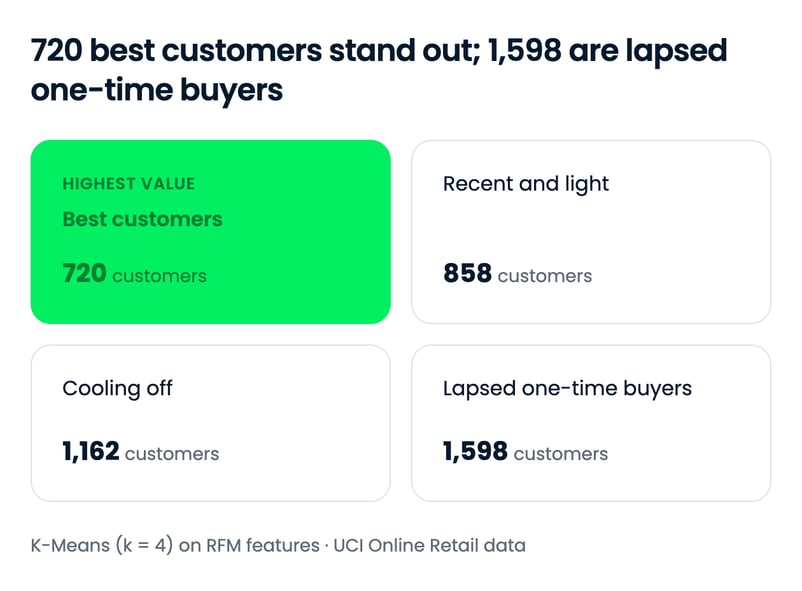
The silhouette score peaks at k = 2, but 2 segments mostly split active customers from lapsed ones, which a marketing team can't do much with. k = 4 scores the same as k = 3 and splits the active customers into big spenders and newcomers, so I'll use it and profile each cluster:
kmeans = KMeans(featuresCol="features", k=4, seed=42)
model = Pipeline(stages=[assembler, scaler, kmeans]).fit(rfm_log)
segments = model.transform(rfm_log)
(segments.groupBy("prediction")
.agg(
F.count("*").alias("customers"),
F.round(F.avg("recency"), 1).alias("avg_recency"),
F.round(F.avg("frequency"), 1).alias("avg_frequency"),
F.round(F.avg("monetary"), 1).alias("avg_monetary"),
)
.orderBy("prediction")
.show())+----------+---------+-----------+-------------+------------+
|prediction|customers|avg_recency|avg_frequency|avg_monetary|
+----------+---------+-----------+-------------+------------+
| 0| 1598| 181.2| 1.3| 326.2|
| 1| 720| 13.2| 13.7| 8072.7|
| 2| 1162| 77.1| 3.9| 1765.2|
| 3| 858| 17.4| 2.3| 613.7|
+----------+---------+-----------+-------------+------------+The four segments read cleanly:
- Cluster 1, best customers (720): bought within the last 2 weeks on average, with about 14 orders and over £8,000 spent each. Retention and loyalty offers go here.
- Cluster 3, recent and light (858): active in the last 3 weeks but with only 2 or so orders. Many are likely new customers worth nurturing toward a second and third order.
- Cluster 2, cooling off (1,162): mid-range spend, but about 11 weeks since their last purchase. A win-back campaign has the best odds here.
- Cluster 0, lapsed one-time buyers (1,598): mostly a single order, around £326, roughly 6 months ago. The largest group and the least valuable.
Cluster numbers are arbitrary labels, and a different seed can reorder them, so always profile the clusters before naming them. To learn how K-Means picks its centroids, see our introduction to k-means clustering, and the pyspark.ml API reference lists every model and transformer. Our Machine Learning with PySpark course covers classification, regression, and model tuning with Pipelines.
Final Thoughts
PySpark comes down to a few ideas: a SparkSession to start, DataFrames for almost everything, lazy transformations that run only when an action needs a result, and the choice of writing each query in Python or SQL. Everything in this tutorial ran in local mode on a laptop, and the same code runs unchanged on a cluster.
A 541,909-row file doesn't need a cluster, and pandas would have handled it. That was deliberate, because the habits that matter on large data (explicit schemas, filtering early, caching what you reuse, and checking explain()) are easier to build on data you can inspect.
From here, these are the best next steps, depending on your goal:
- Practice the DataFrame API with exercises: Introduction to PySpark
- Prepare messy real-world data: Cleaning Data with PySpark
- Keep the syntax at hand: our PySpark cheat sheet
- Prepare for a job interview: Top PySpark interview questions
If you're keen to go further, I recommend our Big Data with PySpark track, which covers data management, feature engineering, machine learning pipelines, and recommendation engines in sequence. For teams, DataCamp for Business offers learning paths for data engineering roles.
PySpark FAQs
What are the prerequisites for learning PySpark?
PySpark 4.3 needs Python 3.11 or later and Java 17 or later (Spark 4.3 runs on Java 17, 21, and 25), with JAVA_HOME pointing to your Java installation. You should be comfortable with basic Python; experience with pandas DataFrames helps, because the PySpark DataFrame API uses similar ideas. You don't need any prior experience with distributed systems.
Is PySpark faster than pandas?
Not on small data. pandas runs in-process with no startup cost, while PySpark spends a few seconds starting the JVM and scheduling tasks, so pandas usually wins on data that fits comfortably in memory. PySpark is faster once the work outgrows one machine's memory or CPU, because it processes partitions in parallel across cores or cluster nodes.
What is the difference between RDDs and DataFrames in PySpark?
An RDD (Resilient Distributed Dataset) is PySpark's low-level structure: a distributed collection of arbitrary Python objects that you process with your own functions. A DataFrame organizes data into named, typed columns, like a pandas DataFrame, and Spark's Catalyst optimizer turns DataFrame queries into efficient execution plans. Use DataFrames for almost all new code, and RDDs only for unstructured data or fine-grained control over partitioning.
How do I run PySpark in a Jupyter Notebook?
Install Java 17 or later, then run pip install "pyspark[sql]" in the environment your notebook uses. Create a SparkSession in the first cell:
from pyspark.sql import SparkSession
spark = SparkSession.builder.appName("MyNotebook").getOrCreate()If you'd rather skip the local setup, DataLab and Databricks notebooks come with PySpark preinstalled.
When should I use PySpark instead of pandas?
Use PySpark when your data doesn't fit in one machine's memory, when a job needs to run on a cluster or a platform like Databricks, or when you're building pipelines that will grow beyond a laptop. For exploratory analysis on data that fits in memory, pandas is simpler and starts instantly. PySpark code written locally runs unchanged on a cluster, so starting with it makes sense if scale-up is likely.
What is lazy evaluation in PySpark?
Lazy evaluation means PySpark doesn't run transformations such as filter() or withColumn() when you call them. It records them in a plan and runs that plan only when an action, such as count(), show(), or write, needs a result. Waiting lets Spark optimize the whole chain, for example by pushing filters down into the file scan.
How do I run SQL queries in PySpark?
Register a DataFrame as a temporary view with df.createOrReplaceTempView("sales"), then query it with spark.sql("SELECT ... FROM sales"). The result is a regular DataFrame, so you can mix SQL and DataFrame code freely. Both compile to the same optimized plan, so neither is faster.
Do I need Hadoop to run PySpark?
No. pip install pyspark bundles the Spark runtime, which runs in local mode on your machine without Hadoop. You only need Hadoop components if you read from HDFS or run Spark on a YARN cluster.

Natassha is a data consultant who works at the intersection of data science and marketing. She believes that data, when used wisely, can inspire tremendous growth for individuals and organizations. As a self-taught data professional, Natassha loves writing articles that help other data science aspirants break into the industry. Her articles on her personal blog, as well as external publications garner an average of 200K monthly views.



PySpark is the Python API for Apache Spark. You write DataFrame code or SQL in Python, and Spark splits the work across every CPU core on your laptop or every machine in a cluster. I reach for it when a dataset no longer fits comfortably in pandas, or when the same job has to run on a cluster later without a rewrite.
In this PySpark tutorial, I'll install PySpark 4.3, create a SparkSession, and explain the two ideas that trip up most newcomers: RDDs versus DataFrames, and lazy evaluation. Then we'll work through the operations you'll use every day (select, filter, groupBy, join, and Spark SQL) on a 541,909-row e-commerce dataset, and finish with a K-Means customer segmentation model built with the
pyspark.mlPipeline API.If you'd like guided exercises alongside this tutorial, our Introduction to PySpark course covers the same ground. For a longer learning plan, see our guide How to Learn PySpark From Scratch.
TL;DR
pip install "pyspark[sql]"; PySpark 4.3 needs Python 3.11+ and Java 17+.SparkSession, and DataFrames (not RDDs) are the default API.count()orshow().pyspark.mlPipelines chain feature preparation and models like K-Means into one object.What Is Apache Spark?
Apache Spark is an open-source engine for distributed data processing. It splits a dataset into partitions, processes them in parallel across a cluster, and keeps intermediate results in memory instead of writing them to disk between steps.
That in-memory design is the main reason Spark replaced Hadoop MapReduce for most batch workloads (we compare the two in Hadoop vs Spark). Spark started at UC Berkeley's AMPLab in 2009, became a top-level Apache project in 2014, and reached version 4.3 on October 30, 2026.
One engine covers several workloads through its built-in libraries:
pyspark.ml) for distributed machine learningFor a closer look at how the driver, cluster manager, and executors divide the work, see our Apache Spark architecture guide.