Apache Spark Architecture: A Guide for Data Practitioners

Have you ever tried to debug a Spark job that suddenly failed and figured out that you are completely lost because of how deep the Spark rabbit hole goes? 

When I first worked with Apache Spark, I thought I just had to write a few PySpark transformations and Spark would “magically” scale across the cluster. I was wrong. Spark's performance depends entirely on understanding what’s happening behind the scenes.

This guide is for anyone who doesn’t want to treat Spark like a black box. We’ll walk through how Spark’s architecture is designed, from the master-worker model and execution workflow, to its memory management and fault tolerance mechanisms. 

If you want to build fast, fault-tolerant, and efficient big data applications, you’re in the right place!

Foundational Architecture of Apache Spark

Before you write your first line of PySpark, Spark has already made some architectural decisions for you. Spark isn’t just fast because of in-memory computing, but because it’s built on a master-worker architecture that scales and survives real-world chaos like node crashes, Java Virtual Machine (JVM) issues, and inconsistent data volumes.

Let’s break down Spark’s core architecture and why it’s still so powerful and present in modern big data workflows.

Master-worker paradigm

At the core of Spark is the master-worker model. Think of it like this:

• Driver (master): This is the brain of Spark. It runs your main() function, creates the Spark context, handles DAG scheduling, and tells the cluster what to do.
• Executors (workers): These are the muscles. They execute your tasks, keep data in memory, and report back to the driver.

This setup allows you to concentrate on defining transformations, and Spark decides where and how to run them in parallel on the executors. 

What I like about this design is that it’s deployment-agnostic. The same code runs, independent of deploying it on your local machine, in Kubernetes or Mesos. That makes it easy to develop and test it locally, then scale to clusters without rewriting your code.

And here is another powerful benefit of Spark’s driver-worker separation: It improves fault isolation. If a worker node dies while executing a task, Spark can reassign that task to another worker without crashing your application.

Core components

Let’s break down what’s happening inside the driver and the nodes. 

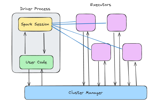
Spark architecture. Image by author.

Spark context

When you call SparkContext() or use SparkSession.builder.getOrCreate(), you’re opening the gateway to all of Spark’s internal magic.

The Spark context:

• Connects to your cluster manager
• Allocates executors
• Keeps track of job status and execution plans

Spark builds a Directed Acyclic Graph (DAG) of transformations behind the scenes. That DAG gets broken down into stages and tasks, then executed in parallel.

The DAG scheduler figures out which tasks can be run together, and the Task scheduler assigns them to executors. Meanwhile, the Block manager ensures data is cached, shuffled, or reloaded as needed. 

This layered design makes Spark incredibly flexible, as you can fine-tune memory, storage, and compute independently.

If you're working with Spark transformations or feature engineering, check out the Feature Engineering with PySpark course to see this architecture in action.

Executor runtime

Executors are where the work gets done.

Each executor runs:

• One or more tasks (threaded)
• A chunk of memory for caching data and shuffling output
• Its own JVM instance, isolated from others

You can configure how much memory each executor gets, how many cores it uses, and whether it should write to disk when memory runs out. 

But, be careful: If you don’t allocate enough memory, you’ll hit out-of-memory errors all the time. However, you should also avoid allocating too much memory, as this wastes resources. Monitoring and tuning are essential here.

Execution Workflow: From Code to Cluster

Writing PySpark code feels quite simple. You filter a DataFrame, do a join, aggregate something, and hit run. But behind that clean API, Spark is quietly spinning up an execution engine that can spread work across several nodes. 

Let’s walk through what happens behind the scenes.

Logical to physical plan conversion

Here’s what most Spark users don’t realize at first: When you write PySpark code, you’re not running anything immediately. You’re building a plan, and Spark’s Catalyst Optimizer takes that plan and transforms it into an efficient execution strategy.

It works in four phases:

1. Analysis: Spark resolves column names, data types, and table references, making sure everything is valid.
2. Logical optimization: This is where Spark applies rules like predicate pushdown and constant folding. It optimizes filters and combines projections.
3. Physical planning: Spark considers multiple execution strategies and picks the most efficient one (based on data size, partitioning, etc.).
4. Code generation: Finally, it uses whole-stage code generation to produce JVM bytecode. 

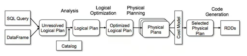
Spark’s Catalyst Optimizer. Image by Databricks.

So that chain of .select(), .join(), and .groupBy() is not just running line by line. It’s getting analyzed, optimized, and compiled into something that runs fast on a cluster.

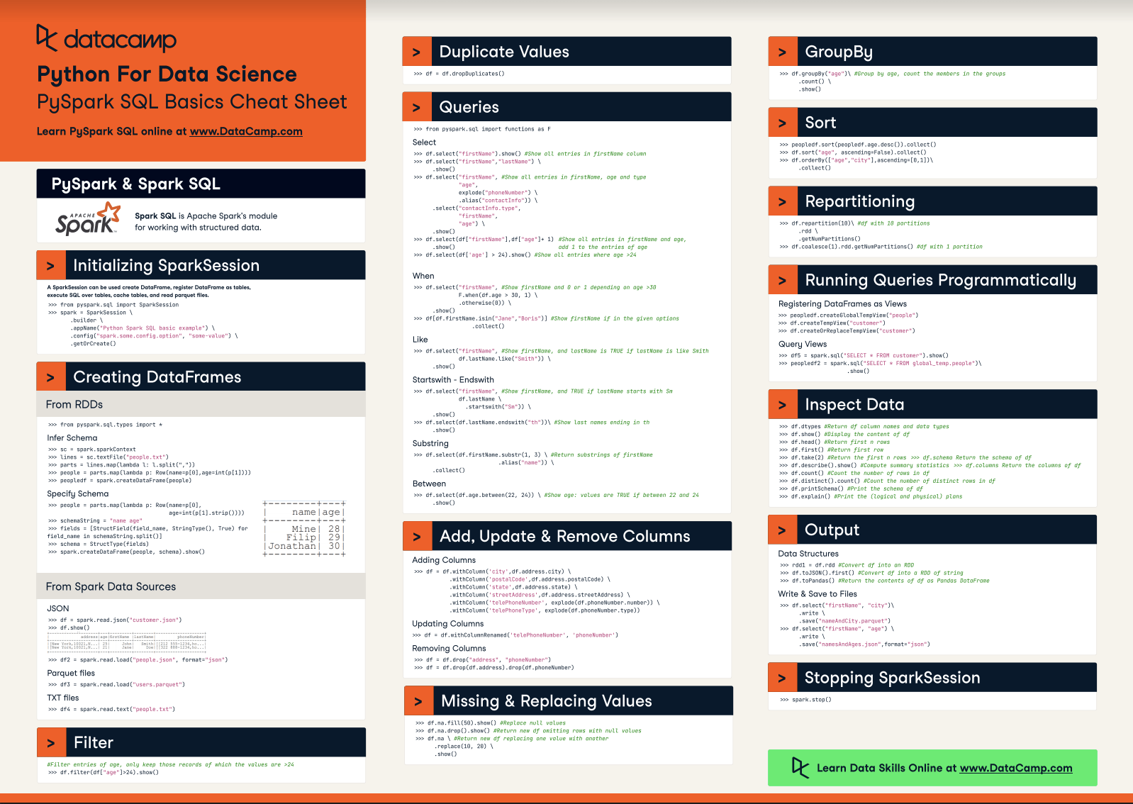
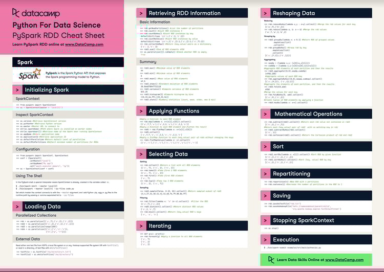
Check out this PySpark Cheat Sheet if you want a cheat sheet for the most useful PySpark commands.

DAG scheduler & stage creation

When the plan is finished, the DAG scheduler takes over.

It breaks the job down into stages based on shuffle boundaries, where Spark decides what happens sequentially and what can be executed in parallel.

There are two main types of stages:

• ShuffleMapStage: This involves a shuffle, which is usually caused by wide transformations like groupBy() or join(). The data is then partitioned and sent across the network. This stage type is required to compute the ResultStage.
• ResultStage: These stages produce output, like writing to disk or returning results to the driver.

One key thing I’ve learned is to minimize shuffles. A shuffle has to take place before a stage finishes and is expensive. You need to understand where they occur in your DAG and whether you can optimize your code further to reduce the number of shuffles. 

Task execution lifecycle

Once the DAG scheduler has created all stages, they can be executed on the different executors. 

The task execution lifecycle looks something like this:

1. Task serialization: The driver serializes task instructions and sends them to the executors.
2. Shuffle write phase: Spark writes the partitioned output to the local disk.
3. Fetch phase: Executors on the next stage fetch the relevant shuffle files from others across the cluster.
4. Deserialization and execution: Executors deserialize the data, run your logic, and potentially cache or write results.
5. Garbage collection: JVM automatically reclaims memory that is no longer being used by Spark applications. This step is essential to prevent memory leaks and ensure that Spark applications run smoothly.

A slight hint from my own experience: if your Spark job hangs after running fine before, it’s often because of garbage collection or shuffle fetch delays. Always check your code and ensure that you understand Spark’s architecture so that you can optimize these topics effectively.

Memory Management Architecture

Spark’s memory management is a very complex topic and can cost you hours of debugging if you don’t understand it. 

Let’s therefore take a look at how Spark manages memory under the hood so that you are aware of it and can avoid hours of debugging slow code or out-of-memory errors.

Unified memory model

Before Spark 1.6, memory was strictly divided between execution (for shuffles and joins) and storage (for caching). That changed with Spark 1.6, introducing the unified memory model. 

In the unified memory model, data is split into three key pools:

• Reserved memory: A small amount of memory is used for Spark internals and the system. 
• Spark memory: This is used for storing execution data and for caching. It is dynamically shared. If your job needs more memory for shuffles and less for caching (or vice versa), Spark adapts.
• User memory: Space for user-defined data structures required for executing user code within Spark applications.

The Spark memory pool is further divided into two pools:

1. Executor memory: Stores temporary data needed during stages of processing tasks (e.g. shuffles, joins, aggregations, …). 
2. Storage memory pool: Used for caching data and storing internal data structures. 

This elasticity allows Spark to be more flexible with unpredictable data volumes. 

However, this also means losing a bit of control when you don’t know what's going on. For example, if you cache() a large DataFrame but also have expensive aggregations in the same stage, Spark might evict your cached data to make room for the shuffle.

Off-heap & columnar storage

In Spark’s off-heap and columnar storage, the Tungsten engine comes into play. 

Tungsten introduced several optimizations that improved Spark's performance:

• Off-heap memory management: Spark now stores some data outside the JVM heap, reducing garbage collection overhead and making memory management more predictable.
• Binary format storage: Data is stored in a compact, cache-friendly binary form, which improves CPU usage and enables vectorized execution.
• Cache-aware algorithms: Spark can now use CPU caches more effectively, avoiding unnecessary reads from RAM or disk.

And if you're working with DataFrames, you’re already using these optimizations under the hood. That’s one of the reasons I push people to use DataFrames and SQL APIs over raw RDDs. You get the full power of Catalyst and Tungsten without any extra tuning.

If you're working with data cleaning pipelines, you'll see this in action in Cleaning Data with PySpark.

Fault Tolerance Mechanisms

If you work with distributed systems, you know one thing for a fact: They fail. Nodes crash. Network errors happen. Executors run out of memory and shut down.

But Spark is built to handle these issues and ensures that your jobs still succeed. 

Let’s dive deeper into how Spark ensures that your jobs still succeed, even if some instabilities occur.

RDD lineage tracking

Resilient Distributed Datasets (RDDs) are the fundamental data structure in Spark. And they are called resilient for a reason. 

Spark uses lineage to ensure that each RDD can be recomputed in the event of a node failure and data loss. 

So when a node fails, Spark simply recomputes the lost data using the lineage graph. 

Here is how it works in practice: 

• Narrow dependencies (like map() or filter()): Spark only needs the lost partition to recompute.
• Wide dependencies (such as groupBy() or join()): Spark may need to fetch data across multiple partitions, as it may require the output of several stages. 

Lineage avoids the need to handle failures manually. However, if your lineage graph becomes too long, as it may contain hundreds of transformations, recomputing lost data becomes expensive. That’s where checkpointing comes into play.

Checkpointing & write-ahead logs

When you encounter complex workflows or streaming jobs, Spark cannot depend solely on lineage. That’s where checkpointing comes into play.

You can call rdd.checkpoint() to persist the current RDD state to a reliable storage location (like HDFS). 

Spark then truncates the lineage. If an error occurs, it reloads the data directly instead of recomputing it.

In structured streaming, Spark also uses write-ahead logs (WALs) to ensure data isn’t lost in transit. 

This is what makes it so stable: 

• Reliable receivers: They write incoming data to logs before processing.
• Executor heartbeats: These regular signals confirm that executors are alive and healthy.
• Checkpoint directories: For streaming jobs, they hold offsets, metadata, and output state so you can resume where you left off.

Checkpointing is optional for batch processing jobs, but required for streaming pipelines. 

Assume you had a Spark job that failed after running 10 hours, but you can resume where you left off, thanks to checkpointing and WALs. 

Advanced Architectural Features

By now, you’ve seen how Spark processes jobs and handles memory and failure.

In this section, we’re diving into some of the advanced architectural upgrades that make Spark more dynamic, more real-time, and more adaptable.

Adaptive query execution (AQE)

AQE is introduced in Spark 3.0 and enhances query performance by dynamically adjusting execution plans at runtime based on statistics collected during execution.

Features of AQE include:

• Dynamically switch join strategies: If your broadcast join isn’t going to fit in memory, AQE switches to a sort-merge join.
• Coalesce shuffle partitions: Merge tiny shuffle partitions into larger ones, which reduces the overhead.
• Handle skewed data: AQE can split skewed partitions to balance out execution time.

This feature is a game-changer, as it enables jobs that previously required manual tuning and trial-and-error to adapt in real-time.

Just make sure to enable it explicitly via the configuration (spark.sql.adaptive.enabled = true). And if you’re running on Spark 3.0+, there’s no reason not to.

Structured streaming architecture

Structured Streaming takes Spark’s engine and extends it into the real-time domain, without requiring you to learn a whole new API.

Behind the scenes, it still applies micro-batching. But it handles:

• Offset management: Spark tracks exactly which data has been read from your source (Kafka, socket, file, etc.). This provides strong exactly-once guarantees when configured correctly.
• Watermarking: With time-based aggregations, Spark uses watermarks to decide when late data is too late to include. This is critical for event-time processing.
• State stores: When you do windowed aggregations or streaming joins, Spark maintains state across micro-batches. This state is stored on disk and checkpointed to avoid data loss.

What’s powerful here is how streaming feels like batching. You write a groupBy() or a filter() and Spark handles everything else, making streaming analytics accessible without a specialized toolchain.

Security Architecture

If you’re running Spark in production, especially in finance, healthcare, or similar business areas, you need to know how Spark handles authentication, encryption, and auditability.

So let’s dive deeper into these topics and how Spark takes care of them.

Authentication & encryption

Spark has many security features that you must first enable. But once enabled, Spark offers a solid toolbox for secure communication and authentication: 

• Authentication (SASL): Spark uses the Simple Authentication and Security Layer (SASL) to verify that only authorized users and services can submit jobs or connect to the cluster.
• Encryption in transit (AES-GCM, SSL/TLS): Spark encrypts communication between nodes using AES-GCM (authenticated encryption) or TLS. This protects job data from being sniffed, especially important in multi-tenant or cloud environments.
• Kerberos integration: If you’re running on Hadoop/YARN, Spark integrates with Kerberos for secure user authentication. This ties your Spark jobs directly into enterprise identity and access management systems.
• UI access control: The Spark Web UI can leak sensitive info (like logs, input paths, SQL queries), so set spark.acls.enable=true and spark.ui.view.acls and spark.ui.view.acls.groups to restrict it.

You can check all security features in the official documentation of Spark. Check it out and ensure that you enable the features you need to secure your Spark applications.

Audit & compliance

Logging who did what and when is also critical. 

Spark supports: 

• Event logging: When enabled (spark.eventLog.enabled=true), Spark records every job, stage, and task event to disk. You can use these logs to replay job history or meet audit requirements.
• Role-based access control (RBAC): Spark doesn’t provide RBAC, but if you’re using Spark through a platform like Databricks, EMR, or OpenShift, you’ll usually get RBAC at the infrastructure layer. Spark submits jobs using a defined identity, which controls access to both data and compute resources.
• Data masking and access control at source: Spark reads from many sources (Parquet, Delta Lake, Hive, etc.), and your access control should be enforced there.

Performance Optimization Patterns

Spark is quite powerful and fast, and it can be optimized to be even faster if you know where to make the necessary adjustments. 

There are several areas where you can try to optimize to get the most out of Spark. So let’s dive deeper into each area.

Shuffle optimization

If Spark has a weak point, it's the shuffle. Shuffles happen when data needs to be moved between partitions, typically after wide transformations like groupByKey(), distinct(), or join().

And when shuffles go wrong, you can get massive disk I/O, long garbage collection pauses, or skewed tasks that never finish. 

Here’s how you can improve shuffles:

• Prefer reduceByKey() over groupByKey(): reduceByKey() aggregates locally before shuffling. groupByKey() sends everything over the network.
• Repartition smartly: Use .repartition(n) to increase parallelism, or .coalesce(n) to reduce it. Don’t leave it up to Spark’s default partitioning.
• Use broadcast joins (wisely): If one dataset is small enough, broadcast it to all workers. Set spark.sql.autoBroadcastJoinThreshold to control the size limit.
• Avoid collect(): Avoid it when possible, as pulling data to the driver kills performance.

Memory configuration guidelines

Tuning Spark’s memory can be quite a science, but you can use the checklist below to make it easier:

• Allocate sufficient memory: Start with at least 6 GB of memory for the Spark cluster and adjust based on your specific needs.
• Consider Spark memory fraction: By default, 60% is the memory fraction in Spark. Increase it if your applications rely heavily on DataFrame/Dataset operations or if you need more user memory. 
• Use the correct number of cores per executor: Usually, 3-5 is optimal. Too few leads to underutilization, while too many lead to task contention.
• Enable dynamic allocation (if supported): Spark can scale executors up/down based on the workload. 

spark.dynamicAllocation.enabled=true
spark.dynamicAllocation.minExecutors=2
spark.dynamicAllocation.maxExecutors=20

• Adjust storage fraction: If you need more caching, increase the spark.memory.storageFraction value.
• Monitor and profile memory usage: Utilize tools such as the Spark UI or VisualVM to track memory consumption and pinpoint bottlenecks.

Adjusting the memory configuration can help significantly. I once reduced a 30-minute job to 8 minutes by adapting the memory configuration, without changing a single line of code.

Cluster sizing formulas

This is the part most teams get wrong, because they guess the cluster size instead of estimating it correctly. 

But you can do better by using the formulas below: 

1. Determine the number of partitions: 
• Calculate the number of partitions needed based on your data size and desired partition size. 
• A standard guideline is to have one partition per 128 MB to 256 MB of uncompressed data.
• Formula: Number of Partitions = Round up(Total Data Size ÷ Partition Size).
2. Calculate the total number of cores: 
• The number of cores needed should be sufficient to process all partitions in parallel.
• Formula: Total Cores = Round up(Number of Partitions ÷ Partitions per Core).
3. Determine memory per executor: 
• Calculate the amount of memory each executor needs based on its cores, partition size, and overhead.
• Formula: Memory per Executor = Base Memory × (1 + Overhead Percentage).
4. Calculate the number of executors: 
• Determine the number of executors based on the total number of cores and cores per executor.
• Formula: Number of Executors = Round up(Total Cores ÷ Cores per Executor).
5. Calculate total memory: 
• Calculate the total memory needed for the cluster based on the number of executors and memory per executor.
• Formula: Total Memory = Number of Executors × Memory per Executor.

For example: 

• Input: 500GB of data and a partition size of ~128MB
• Partitions: ~4,000 partitions
• Cores: 4,000 partitions / 4 partitions per core = 1,000
• Memory per executor: Assume 8 GB per executor and 20% overhead. 8 GB * 1.20 = 9.6 GB
• Executors: 1,000 cores / 4 cores per executor = 250 executors
• Total memory: 250 executors * 9.6GB = 2,400 GB

But remember: This is only an estimate. You can use it as a starting point and then further optimize through profiling.

Emerging Architectural Trends

Spark has been around for a decade, but it remains quite up to date. It’s evolving faster than ever, thanks to cloud-native platforms, GPU acceleration, and tighter ML integration.

If you’re using Spark today the same way you did three years ago, you’re probably leaving performance on the table and missing out on great new features.

Let’s take a look at some of the newest ones.

Photon engine (Databricks)

If you work with Databricks, you’ve probably already worked with and heard of Photon.

If you want to learn more about Databricks, I recommend the Introduction to Databricks course.

Photon is the next-generation engine on the Databricks Lakehouse platform that provides speedy query performance at low cost. It is compatible with Spark APIs, so you don’t need to adapt your Spark code to make use of it. 

It helps to significantly boost your SQL and PySpark code.

Photon includes the following features: 

• Vectorized execution: Photon processes data in columnar batches, leveraging SIMD (Single Instruction, Multiple Data) CPU instructions to perform operations on multiple values simultaneously. Traditional Spark uses row-by-row execution and relies heavily on the JVM for memory allocation and garbage collection.
• C++ runtime (no JVM overhead): No Java garbage collection, which can be a bottleneck in large Spark jobs. Memory is managed with precision in C++.
• Improved query optimizations: Photon integrates deeply with Spark’s Catalyst Optimizer, but it also includes its optimizations during execution (like runtime filtering, adaptive code paths, join and aggregation optimizations). 
• Hardware acceleration: Support for modern hardware (like NVIDIA GPUs, AVX-512 instruction sets for Intel CPUs, Graviton (ARM) processors on AWS). 

Serverless Spark

Serverless is fantastic, as it means you don’t have to manage clusters, pre-provision resources, and you only pay for the time Spark is running. 

And serverless for Spark is already live in services like Databricks Serverless, AWS Glue, and GCP Dataproc Serverless.

And here’s why it is incredible:

• Automatic scaling: The platform scales compute based on your job’s actual needs, meaning you don’t need to guess how many nodes you need.
• Cost-effectiveness: You only pay for what you use. No more paying for idle servers. 
• Simplicity: No need to deal with cluster setup, configuration, or maintenance, as this is taken care of for you.
• Performance: Faster execution times are possible, as the configuration and setup are optimized for you.

Serverless Spark is ideal for interactive analytics, ad-hoc jobs, or unpredictable workloads.

But be careful: long-running, consistent pipelines may still be cheaper on fixed clusters. Always measure both cost and latency.

MLflow integration

If you’re doing machine learning at scale and you aim at bringing models into production, Spark alone isn’t enough. You need MLOps principles, such as experiment tracking, model versioning, and reproducibility. That’s where MLflow fits in. 

MLflow now integrates with Spark and brings a full MLOPs stack to your pipelines.

You can: 

• Track experiments: Log parameters, metrics, and artifacts from Spark ML jobs using mlflow.log_param() and mlflow.log_metric().
• Version models: Save models from pyspark.ml or sklearn directly into MLflow’s model registry.
• Serve models: Deploy trained models to REST endpoints using MLflow’s model serving.

You don’t need to switch tools. You continue to use Spark for training, feature engineering, and scoring, while utilizing MLflow for MLOPs tasks.

Conclusion

If you don’t know much about Spark, it is like a giant black box. You write some PySpark code, hit run, and hope it works. 

Sometimes that worked well for me, sometimes it led to long debugging sessions and figuring out what went wrong. 

It wasn't until I started to look behind the scenes that things made sense to me. And it took quite a while for me to understand what’s going on.

Here’s what I would focus on if I were starting from scratch again: 

• Learn how Spark breaks your code into jobs, stages, and tasks.
• Understand memory.
• Watch out for shuffles.
• Start small and run things in local mode. Get your hands dirty.

That’s precisely what we learned in this article.

If you want to keep learning, here are some beginner-friendly resources I’d recommend:

• Introduction to PySpark: A great hands-on starting point if you're still getting comfortable.
• Cleaning Data with PySpark: Learn to clean data, because real-world data is always messy.
• The Top 20 Spark Interview Questions: This is not just for interviews, but to deepen your understanding.
• Top 4 Apache Spark Certifications in 2025: In case you want to get your skills acknowledged via certifications.