Mastering PySpark’s groupBy for Scalable Data Aggregation

In the world of big data, we rarely stare at raw data. To make data more digestible, grouping and aggregating data is a common and powerful operation. When working with distributed systems like Apache Spark and Python, having PySpark’s groupBy function allows us to gather and summarize our distributed data. It mirrors the functionality of SQL’s GROUP BY clause, but is designed to handle distributed data processing over massive datasets efficiently.

PySpark’s groupBy allows users to partition data based on a variety of columns, which can then be aggregated into various measures like sums, averages, and so on. To do this efficiently, PySpark follows the split-apply-combine paradigm:

1. Split the data into groups based on criteria,
2. Apply aggregation or transformation logic to each group,
3. Combine the results into a new DataFrame.

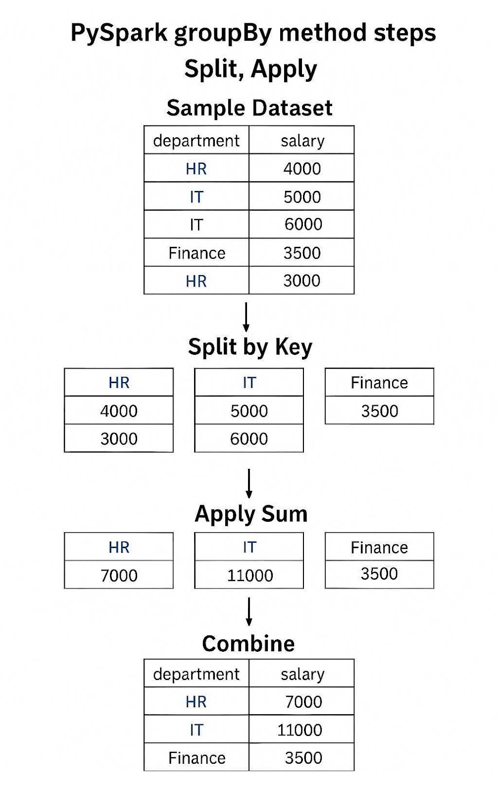
Example of PySpark’s groupBy() method applying Sum

PySpark leverages lazy evaluation, meaning operations like groupBy are only computed when actions (like show() or collect()) are called. Instead, PySpark first builds an initial DAG (Directed Acyclic Graph) that is refined for performance. This helps Spark optimize the query plan before execution. 

If you haven’t had a chance to work with PySpark, I highly recommend going over some Big Data Fundamentals with PySpark.

Creating a PySpark DataFrame

First things first, we need to have a PySpark DataFrame. If you need a refresher on the various PySpark commands, check out this great PySpark DataFrame Cheatsheet. 

We’ll go over some of the key steps and commands that will help us get going with PySpark. Before getting started, make sure you have PySpark installed in your Python environment as well as Java and Java JDK. If you need assistance, follow this guide on getting started with PySpark.

Initiating SparkSession

Step one is getting your PySpark running!

from pyspark.sql import SparkSession

# Start a SparkSession
spark = SparkSession.builder \
    .appName("GroupByExample") \
    .getOrCreate()

Sample DataFrame for GroupBy

Let’s build a sample DataFrame for us to work with.

from pyspark.sql import Row

data = [
    Row(department="Sales", employee="Alice", salary=5000),
    Row(department="Sales", employee="Bob", salary=4800),
    Row(department="HR", employee="Carol", salary=4000),
    Row(department="HR", employee="David", salary=3900),
    Row(department="IT", employee="Eve", salary=6000)
]

df = spark.createDataFrame(data)
df.show()

Output:

	+----------+--------+------+
	|department|employee|salary|
	+----------+--------+------+
	|     Sales|   Alice|  5000|
	|     Sales|     Bob|  4800|
	|        HR|   Carol|  4000|
	|        HR|   David|  3900|
	|        IT|     Eve|  6000|
	+----------+--------+------+

What is PySpark GroupBy?

PySpark groupBy is a transformation used to split the data into groups based on one or more columns, which can then be aggregated or transformed independently.

Basic syntax and examples

Using the groupBy method is simple; you can call it on your dataframe of interest. You can use it on any column type as long as it’s appropriate to partition on. For instance, you might want to avoid floats.

grouped = df.groupBy("department")

This creates a GroupedData object, which is not a DataFrame itself. It does tell Spark to generate how it would begin to partition the data. Once you have this GroupedData object, you can apply aggregations .count() or .sum() to obtain a new DataFrame.

grouped.count().show()

Parameters and return values

The only parameter for the method is *cols which accepts column names, column expressions, column ordinals (int), or a list of columns. As long as the column is something you wish to partition by, you are able to use it in the operation. It will always return a GroupedData object.

# grouping by column name like above
	df.groupBy("department")

# grouping by column expression
	df.groupBy(df.department)

#grouping by column ordinal
	df.groupBy(1)

#grouping by list of columns, you can mix the methods!
	df.groupBy(["department", 2])

GroupBy on single and multiple columns

As shown above, you can group on a single or multiple columns. A single column is great for when you are only interested in a single axis, like departments or years. Multiple columns are great if you want to get more layers of detail, for instance, specific salespeople in different departments, or specific months within a year.

# grouping by single column
	df.groupBy("department").sum(“salary”).show()

#grouping by multiple columns
	df.groupBy(["department", 2]).sum(“salary”).show()

As you have probably noticed, the groupBy method works very similarly to SQL’s GROUP BY statements. We will show a way to use that language in PySpark as well later.

Aggregation Functions and Techniques

PySpark supports a wide array of built-in aggregation methods to work with grouped data. If you are familiar with SQL, you will be familiar with many of them such as count(), sum(), avg(), and so on. You can check out our aggregate functions in SQL guide for a refresher. 

Built-in aggregation functions

Let's go over the built-in aggregation functions:

• count(): counts the number of records in this partition
• sum(): summarizes the total of numerical values
• avg(): average the numerical values
• min(): returns the smallest value of the partition
• max(): returns the largest value of the partition

In addition to the aggregation functions, you can attach the .alias() method to rename the columns so that they are more easily understandable. We will show an example below.

Multiple aggregations with agg()

Instead of performing each aggregation independently, you can do multiple aggregations at once by using the agg() method. Each aggregation will create a new column in your dataframe. It also reduces the need for multiple groupBy calls, which improves performance. We do not need to aggregate on the same column with agg(), you can define a different column for each aggregation function.

# After already starting your session
from pyspark.sql import functions as sf

df.groupBy("department").agg(
    sf.count("employee").alias("employee_count"), 
    sf.avg("salary").alias("avg_salary"),
    sf.max("salary").alias("max_salary")
).show()

Output:

+----------+--------------+----------+----------+
|department|employee_count|avg_salary|max_salary|
+----------+--------------+----------+----------+
|     Sales|             2|    4900.0|      5000|
|        HR|             2|    3950.0|      4000|
|        IT|             1|    6000.0|      6000|
+----------+--------------+----------+----------+

Advanced aggregation patterns

The benefit of PySpark is the ability to use some more advanced aggregation patterns, such as pivoting your data, rolling up, and creating data cubes. You can also create grouping sets. 

Pivoting

Much like creating a pivot table in Excel, you can pivot your data on different columns in the data. In this instance, we are grouping by department and pivoting on the employee column to see the total salary of each employee. 

This means each row would show the department, and each column would be the employees of that department. You can see how this could be powerful if we had data by year, and we wanted to see how each department did year over year.

df.groupBy("department").pivot("employee").sum("salary").show()

Rollups and cubes

Two very powerful ways to aggregate data are rollup() and cube().  While plain groupby() would show the results for aggregations that exist, rollup()and cube() are both hierarchical structures. Meaning they aggregate data on a more granular level.

For instance, rollup() aggregates from left to right, showing each possible permutation if we were to go through the step-by-step iterations. For each department, we show each person who is in the department and also the final group of those who aren’t.

On the other hand cube() shows all possible  permutations for all aggregated columns, so for every department separately, every employee separately, and every combination of both. 

To summarize:

• Rollup creates hierarchical subtotals following the order of columns.
• Cube generates subtotals for every possible combination of the specified columns.

You can see an example in the code and output below:

rollup() Code:

# using rollup
df.rollup("department", “employee”).sum("salary").show()

rollup() Output:

+----------+--------+-----------+
|department|employee|sum(salary)|
+----------+--------+-----------+
|      NULL|    NULL|      23700|
|     Sales|   Alice|       5000|
|     Sales|    NULL|       9800|
|     Sales|     Bob|       4800|
|        HR|   Carol|       4000|
|        HR|    NULL|       7900|
|        HR|   David|       3900|
|        IT|     Eve|       6000|
|        IT|    NULL|       6000|
+----------+--------+-----------+

cube() Code:

#using cube
df.cube("department", "employee").sum("salary").show()

cube() Output:

+----------+--------+-----------+
|department|employee|sum(salary)|
+----------+--------+-----------+
|      NULL|   Alice|       5000|
|      NULL|    NULL|      23700|
|     Sales|   Alice|       5000|
|     Sales|    NULL|       9800|
|     Sales|     Bob|       4800|
|      NULL|     Bob|       4800|
|      NULL|   Carol|       4000|
|        HR|   Carol|       4000|
|        HR|    NULL|       7900|
|        HR|   David|       3900|
|      NULL|   David|       3900|
|        IT|     Eve|       6000|
|        IT|    NULL|       6000|
|      NULL|     Eve|       6000|
+----------+--------+-----------+

Grouping sets

Grouping sets allow you to define multiple levels of aggregation. In this example, I am aggregating on the department and employee level, the department level, and all levels to get the total salary.

You’ll see the syntax is a little different for the groupingSets() method. You first define the list of sets [(“department”, “employee”), (“department”, ), ()] where the first set is department and employee, the second set is just departments, and the last set of () means all. 

You then define the columns of aggregation within the sets. The rest of it is written as normal using .agg().

df.groupingSets([("department", "employee"), ("department",), ()], "department","employee").agg(sf.sum("salary")).sort("department","employee").show()

Output: 

+----------+--------+-----------+
|department|employee|sum(salary)|
+----------+--------+-----------+
|      NULL|    NULL|      23700|
|        HR|    NULL|       7900|
|        HR|   Carol|       4000|
|        HR|   David|       3900|
|        IT|    NULL|       6000|
|        IT|     Eve|       6000|
|     Sales|    NULL|       9800|
|     Sales|   Alice|       5000|
|     Sales|     Bob|       4800|
+----------+--------+-----------+

Custom aggregation functions

Finally, we can create custom aggregation functions using User Defined Functions (UDFs) in PySpark. There are two ways: udfand pandas_udf. Both of these allow you to create your own custom functions with pros/cons to both.

The standard spark udf allows you to create Spark-native functions. That means the syntax and data types must work in Spark natively. While this does limit some of what can be done in the UDF, this allows you to take full advantage of the distributed computational power of Spark and is better for larger datasets.

from pyspark.sql.functions import udf
from pyspark.sql.types import IntegerType

@udf(returnType=IntegerType())
def bonus(salary):
    return int(salary * 0.1)

df.withColumn("bonus", bonus(df.salary)).show()

On the other hand, pandas_udf allows you to create more Pythonic custom functions. You are now only beholden to what’s possible in Pandas and not just Spark. 

However, that means you are not able to use the distributed computational power of Spark, and you rely on local computation. This is a better fit for smaller to medium-sized datasets.

import pandas as pd
from pyspark.sql.functions import pandas_udf

@pandas_udf("double")
def salary_bonus(s: pd.Series) -> pd.Series:
    return s * 0.1

df.withColumn("bonus", salary_bonus(df.salary)).show()

Overall, you only really want to use custom functions if and only if there are no better ways to perform the aggregation. Don’t reinvent the wheel! 

Also, if something can be vectorized (like our above functions), then opt to use a vectorized version of the function instead of an aggregation UDF. For more info on groupBy(), read this article that goes more deeply into the split-apply-combine framework with pandas.

Filtering Aggregated Data

In PySpark, you can filter groups based on aggregate metrics post-grouping using the filter() method. In this method, you provide a condition in either Python or SQL expressions. 

On that note, you can also use where() if you’d prefer, as it is simply an alias for filter() and performs the same operation.

You can choose to filter before or after the aggregation. Filtering before will impact the aggregation by limiting what data gets aggregated and can improve performance. 

For instance, maybe we only want to count the number of employees above a certain salary to find the number of “high-salary” employees.

#filter for high salaries
filter_df = df.filter(df.salary > 4000)

#aggregate and find the total of high salary employees
agg_filter_df = filter_df.groupBy("department").agg(sf.count("*").alias("high_salary_emp"))
agg_filter_df.show()

However, filtering after the aggregation would not impact the original aggregation. Maybe we want to count all the employees in a department and only want to see departments above a certain size. This will add an extra layer of processing, but should not greatly increase the computational load.

# creating a dataframe counting the number of employees
agg_df = df.groupBy("department").agg(sf.count("*").alias("num_employees"))

# filtering for departments where there is more than 1 employee
agg_df.where("num_employees > 1").show()

Choose when to filter wisely, as it will impact the accuracy and final result. Filtering before may reduce the final total, whereas filtering after may leave too many in the final answer.

PySpark groupBy Performance Optimization Strategies

While PySpark automatically optimizes the groupBy operation, there are strategies that can further improve the processing speed. Things like minimizing data shuffling, skew mitigation, and execution optimization all play a role in improving groupBy performance.

Shuffle management

groupBy causes a shuffle, which redistributes data across partitions to group similar keys together. Shuffles are network- and disk-intensive, so minimizing or optimizing them is crucial. Here are some key optimization techniques:

• Use repartition() wisely, you can tell PySpark which column the data should be partitioned so that it searches in fewer places for the data
• Adjust spark.sql.shuffle.partitions. By default, PySpark uses 200 shuffle partitions. If the dataset is smaller, you can reduce this number.
• Enable shuffle compression. Compressing shuffles will reduce the amount of network and disk overhead.

Here are some examples of how you can improve shuffle management.

# reduce the number of shuffle partitions
spark.conf.set("spark.sql.shuffle.partitions", "64")  # Adjust based on cluster size

# make sure spark compresses the data
spark.conf.set("spark.shuffle.compress", "true") # compresses network transfer
spark.conf.set("spark.shuffle.spill.compress", "true") # compresses disk spillage

# repartitions the data prior to grouping to optimize aggregation
df.repartition("department").groupBy("department").sum("salary").show()

Skew mitigation techniques

Data skew happens when certain keys appear disproportionately more than others, leading to uneven partition loads and slow tasks. This puts more strain on some workers than others. We can minimize skew and more evenly distribute work by salting, minimizing skewed joins, and broadcast joins for smaller dimensions.

• Salting: Add a column of random numbers that forces even distribution across workers
• Repartitioning to minimize skew, forcing Spark to use a different column for partitioning may result in better workload distribution

# Salting example:

df = df.withColumn("salted_key", sf.rand()) #Create column of random
df = df.repartition(2, 'salted_key') # use this to repartition data
df.groupBy(sf.spark_partition_id()).count().show()

Execution optimization

The logical and physical execution plans of PySpark jobs can be optimized using built-in features. These can enhance the performance of your groupBy aggregations.

• Catalyst optimizer: Spark automatically rewrites inefficient plans, but writing declarative transformations (not procedural loops) helps the optimizer do its job.
• Caching: Caching is useful when the same groupBy result is used multiple times in a pipeline.
• Broadcast joins: Broadcast smaller dataframes to keep them in memory while larger datasets get split up and partitioned to minimize network and disk overhead on the cluster.

grouped_df = df.groupBy("department").sum("salary").cache()
grouped_df.show() # you can cache your intermediate results

# use broadcasting (pseudocode here):
from pyspark.sql.functions import broadcast
df.join(broadcast(smaller_df), "department").show()

For more details on how we can optimize PySpark’s operation, read this article on PySpark Joins to understand some of the under-the-hood mechanics.

Comparative Analysis with RDD Operations

Although the DataFrame API is the recommended interface for most PySpark users due to its higher-level abstraction and performance efficiency, thanks to the Catalyst Optimizer, understanding the Resilient Distributed Dataset (RDD) layer can be valuable, especially for those who want more control or are migrating legacy Spark code. In general though, using the DataFrame or SQL API is going to give you better performance.

The RDD is the core component of PySpark, which all things (including the DataFrame API) is built upon. It tends to work in-memory and handles streaming data somewhat better than the DataFrame API. However, the data is immutable and so cannot be changed once the RDD is created. 

This section compares groupBy in the DataFrame API with its equivalents in the RDD API, analyzing both performance and use-case fit.

Firstly, let's make the dataframe into an RDD.

# Convert DataFrame to RDD of (key, value)
rdd = df[['department','salary']].rdd
rdd.collect()

Now we can perform things like groupByKey() and reduceByKey() on the RDD.  Let’s cover groupByKey() first.

The method groupByKey() shuffles all values with the same key to the same executor and then groups them. Because of this, it can actually take a long time for the data to be shuffled to the right key. This can also lead to data skew.

rdd.groupByKey().mapValues(list).collect()

Instead, we can try the following reduceByKey() method. This method first aggregates on each partition and then moves the data across the network. This minimizes the amount of data being shuffled and as a result works more quickly. 

So, reduceByKey is strongly preferred over groupByKey because it significantly reduces shuffle operations.

So, this aggregates in each partition, then combines the data, and then aggregates it together. This is best for aggregations that bring the keys together, like sum() and max().

from operator import add

rdd.reduceByKey(add).collect()

Performance benefits of DataFrame vs RDD aggregation methods

Here is a table summarizing the benefits of each aggregation method.

The Big Data Fundamentals with PySpark covers programming with RDDs in more detail and describes how they form the backbone of PySpark.

PySpark SQL GROUP BY Query

Another way to perform aggregations in PySpark is to use the SQL API to write statements using SQL. This can be a great way if you are more comfortable writing SQL.

The first step is to create a temporary view using the createOrReplaceTempView() method of the DataFrame. Then you can use spark.sql() to write your statement.

# Create a temporary view using the DataFrame
df.createOrReplaceTempView("employees")

# Write a SQL-like statement
spark.sql("""
    SELECT department, AVG(salary) AS avg_salary
    FROM employees
    GROUP BY department
""").show()

Output:

+----------+----------+
|department|avg_salary|
+----------+----------+
|     Sales|    4900.0|
|        HR|    3950.0|
|        IT|    6000.0|
+----------+----------+

As you can see, it is as easy as writing a normal SQL query. The main time to use the SQL API is for familiarity and an easier time writing your queries. The DataFrame API can often be better as it will provide consistent data types and usually optimizes better. 

You can gain access to DataFrame methods that you would not have access to with the Spark SQL API. For more information on SQL’s GROUP BY, you can read this article on GROUP BY and HAVING in SQL.

Real-World Applications

There are plenty of real-world applications for aggregating your data. In fact, you are almost guaranteed to have to aggregate your data in some way in order for it to be analyzed and shared.

Below, we will provide some examples of different use cases for aggregations. Some of these may be pseudo-code or not exactly applicable to our test dataset, but instead are here to give you an idea of how you might write these aggregations.

Business intelligence

One common theme we’ve discussed is the idea of using groupBy as a means of hierarchical analysis. Imagine we had a column called “revenue” and we were interested in how each department performed. We can group on each department and assess the revenue contribution of each department.

CopyEdit
df.groupBy("department").agg(sum("revenue").alias("total_revenue")).show()

Time-series analysis

Aggregations give you access to window functions. These functions look at a sliding window of data, either a series of rows sequentially or a period of time sequentially. 

We first define a window using the Window object to show what we want to partitonBy and orderBy. We then use this object in the over() method of our aggregation function of choice. For instance, a rolling average would look like sf.avg().over(window).show().

Imagine we wanted to see a rolling average of salaries for each department. We would group by department and order by a new column we can call employeeId. Since employee IDs are often sequential, we can see how the average salary has changed over time. 

from pyspark.sql.window import Window

#Define the window we wish to partition and order by
windowSpec = Window.partitionBy("department").orderBy("employeeId")

#Perform the sf.avg function on the “salary” column over the windowSpec.
df.withColumn("rolling_avg", sf.avg("salary").over(windowSpec)).show()

This is very similar to how we would do window functions in SQL.

Media analytics

Maybe we want to understand multiple different user metrics for our media company. We want things like total watch time and unique videos. We can groupBy() on a user_id column followed by .agg() with different functions such as sum() and countDistinct() for different metrics.

df.groupBy("user_id").agg(
    sf.sum("watch_time").alias("total_watch"), #sum minutes watched
    sf.countDistinct("video_id").alias("unique_views") #count unique videos watched
).show()

PySpark GroupBy Best Practices and Pitfall Avoidance

When aggregating data in PySpark, it’s easy to fall into some pitfalls that lead to poor performance and long run times. Following these best practices helps ensure performance, correctness, and scalability. 

Common pitfalls

Here are some common ways people turn their simple queries into long-running programs.

1. Overusing groupByKey() in RDDs:
• Avoid groupByKey() in RDDs, since its mechanism has PySpark shuffle data across partitions. This can lead to a lot of network and disk overhead.
• Instead, prefer to use reduceByKey() or stick to the DataFrame API.
2. Not handling skewed data:
• When one group dominates (e.g., one department has millions of records), that task can become a bottleneck.
• Use salting or custom partitioning to mitigate this by redistributing the partition workload with the repartition() method.
3. Forgetting to chain aggregation functions:
• Multiple separate lines of aggregation functions like having sum() in one groupBy then count() on the same grouped dataset in a different line leads to inefficient plans by breaking PySpark’s ability to optimize.
• PySpark solves problems using a lazy evaluation model, meaning it generates the entire plan before performing actions. Chaining transformations (e.g., groupBy().agg().filter()) allows the Catalyst optimizer to plan efficiently.
4. Incorrect use of UDFs:
• Python UDFs prevent Spark from optimizing queries fully as Catalyst is unable to optimize for them.
• If possible, use Spark’s built-in functions or pandas UDFs for better performance.
5. Memory mismanagement:
• Aggregations can be expensive and take up a lot of memory. This can lead to memory exhaustion when reusing aggregation results multiple times.
• Monitor memory usage and consider using persist() or cache() when reusing grouped data.

Optimization and efficiency tips

Here are some ways you can optimize your PySpark aggregations to keep them running smoothly!

Null handling

• Aggregating over columns with nulls can yield unexpected results.
• Use na.fill() or na.drop() prior to aggregation.

df.na.fill({"salary": 0}).groupBy("department").sum("salary").show()

Avoid excessive shuffles

• As discussed above, shuffling leads to slow operations. Repartition data logically before grouping to minimize shuffle size.
• Tune spark.sql.shuffle.partitions based on data volume and see what number of partitions works best for your data.

Use explain plans

• Monitor query plans with .explain() to understand physical execution.
• Look for any signs of wide shuffles, broadcast hints, and inefficient scans

df.groupBy("department").sum("salary").explain(True)

Output:

	== Parsed Logical Plan ==
	'Aggregate ['department], ['department, unresolvedalias('sum(salary#600L))]
	+- LogicalRDD [department#598, employee#599, salary#600L], false

	== Analyzed Logical Plan ==
	department: string, sum(salary): bigint
	Aggregate [department#598], [department#598, sum(salary#600L) AS sum(salary)#679L]
	+- LogicalRDD [department#598, employee#599, salary#600L], false

	== Optimized Logical Plan ==
	Aggregate [department#598], [department#598, sum(salary#600L) AS sum(salary)#679L]
	+- Project [department#598, salary#600L]
	   +- LogicalRDD [department#598, employee#599, salary#600L], false

	== Physical Plan ==
	AdaptiveSparkPlan isFinalPlan=false
	+- HashAggregate(keys=[department#598], functions=[sum(salary#600L)], output=[department#598, sum(salary)#679L])
	   +- Exchange hashpartitioning(department#598, 200), ENSURE_REQUIREMENTS, [plan_id=1841]
	      +- HashAggregate(keys=[department#598], functions=[partial_sum(salary#600L)], output=[department#598, sum#681L])
	         +- Project [department#598, salary#600L]
	            +- Scan ExistingRDD[department#598,employee#599,salary#600L]
	

Monitor performance with Spark UI

• Use Spark Web UI to track stages, tasks, and identify slow aggregations or skew.
• You can learn more about the Spark Web UI in this Introduction to Spark SQL in Python course.

Leverage configuration tuning

Spark has many configurations that can be tuned for large  groupBy workloads. Refer to the table below for some key configurations.

Notes and Advanced Implementation Details

For advanced users or those dealing with very large datasets, understanding how groupBy behaves under the hood is essential. Let’s cover some of the finer points of how this method works.

Lazy evaluation and execution plan

All DataFrame operations in PySpark, including groupBy, are lazily evaluated. That means no actual computation happens until an action (like show() or collect()) is triggered. 

This allows the Catalyst optimizer to rearrange, combine, or remove operations to improve performance. Take advantage of this and chain multiple aggregations and methods together so that Spark can create an optimized plan.

Return type and naming collisions

When using groupBy() it returns a GroupedData object. Performing an aggregation function, such as sum() will then return a DataFrame-like object. If using show() it will display the results.

Remember that groupBy().agg() returns a new DataFrame with newly named columns. Always use aliases with the alias()  method to prevent naming collisions and make outputs clearer. If you leave columns with aliasing, it can lead to column name collisions or issues with joins down the line.

from pyspark.sql import functions as F

df.groupBy("department") \

  .agg(

      sum("salary").alias("total_salary"),

      count("*").alias("employee_count")

  )

Aggregate result format

Something to note about PySpark, is that the returned aggregation does not preserve row order. Use orderBy() for predictable outputs and consistent row sorting.

df.groupBy("department").sum("salary").orderBy("department").show()

Version-specific behaviors and limitations

There are some version-specific changes and limitations in each version of PySpark. Catalyst was introduced in 1.3 and significantly improved in 2.0. Some methods were not introduced until later versions of PySpark, such as groupingSets(). 

Here’s a chart that goes over some of the bigger functional changes for PySpark. Make sure you use the right version of Spark and PySpark for what features you need! 

Conclusion

PySpark’s groupBy function is an essential tool for data aggregation in distributed environments. Whether summarizing data by region, computing average metrics, or performing complex multi-level analytics, groupBy provides a scalable and flexible API for handling big data workloads.

Just remember to keep these best practices in mind to minimize runtime and cost:

• Use built-in functions where possible
• Avoid performance pitfalls like excessive shuffling and data skew.
• Leverage Spark's optimizations and profiling tools to fine-tune large jobs.

As PySpark continues to evolve, we can expect even more intelligent optimizations, native support for complex aggregations, and better integration with Pandas and SQL-style syntax. It may even have better integration for larger-scale models. If you have an interest in learning more about PySpark, check out these detailed resources from DataCamp:

• Big Data with PySpark Track
• Top 20 Spark Interview Questions
• Apache Spark Tutorial: ML with PySpark
• Introduction to Spark with sparklyr in R
• Groups: your hub for collaborative data science learning