Track
AI Fundamentals
10 hr
Imagine a system that can identify and neutralize threats it has never encountered before while remembering past invaders to fend them off more efficiently. Your immune system does this every day.
Now, imagine applying this same intelligence level to solving complex computing problems. With artificial immune systems (AIS), we can do just that.
Artificial immune systems are powerful computational models inspired by the human immune system's ability to protect the body from harm.
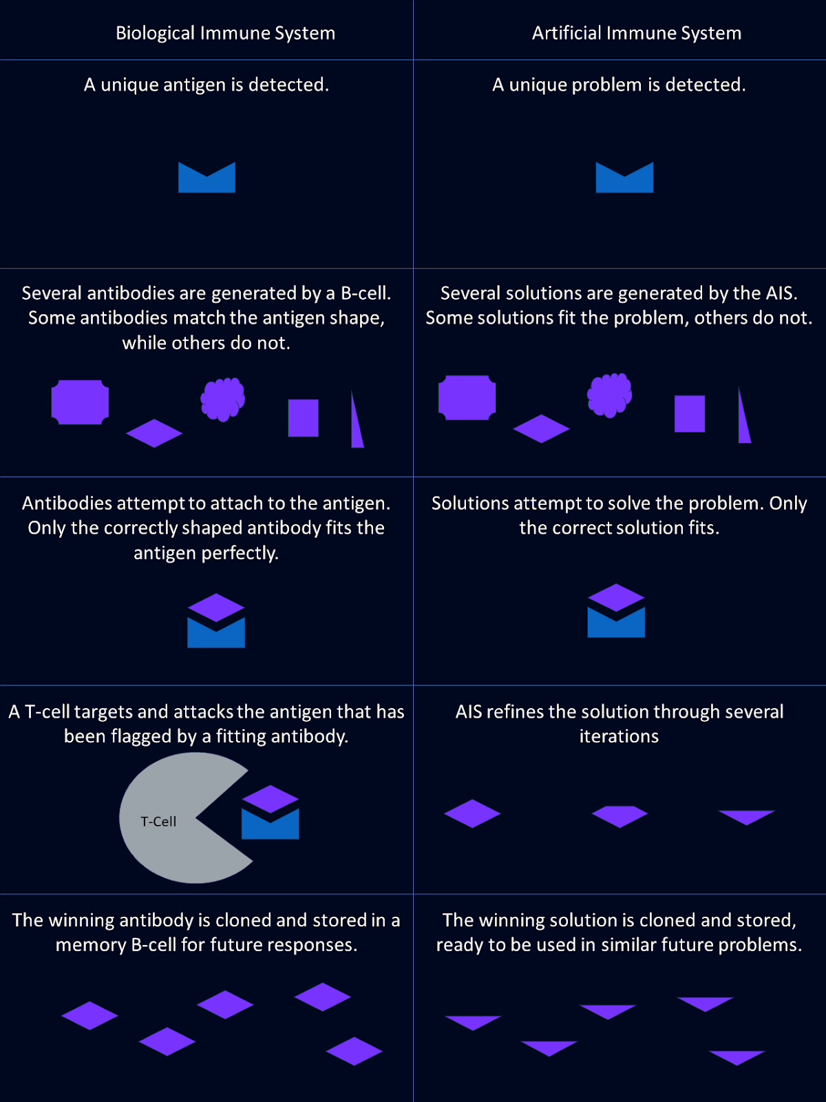
The immune system is our body’s defense mechanism, designed to recognize and neutralize threats like bacteria, viruses, and fungi. It does this through a few key players: antibodies, b-cells, and t-cells.
Antibodies act as the immune system’s identification units. These specialized proteins recognize and attach to specific foreign substances, called antigens, tagging them as threats. Each antibody is unique, designed to match a particular antigen, like a lock and key.
B-cells are the factories that produce antibodies. They are also involved in creating memory cells. These help the body respond faster to previously encountered antigens by remembering which antibodies were helpful last time.
T-cells are the immune system’s enforcers. They detect and destroy cells flagged by antibodies as infected or dangerous, ensuring the threat is swiftly neutralized.
One of the immune system’s most remarkable features is its ability to evolve and improve new antibodies over time. When faced with a new pathogen, the immune system doesn't just respond once. It continuously refines its approach, creating stronger and more effective antibodies to deal with the threat.
Artificial immune systems (AIS) are the implementation of these biological principles into algorithms. AIS mimics the functions of the immune system in problem-solving.
In AIS, antigens represent the problems or challenges to be addressed. These could be anything from detecting anomalies in data to optimizing a solution.
Antibodies in AIS are candidate solutions to these problems. Just like how biological antibodies recognize specific antigens, AIS evolves potential solutions tailored to specific challenges.
The B-cell process in AIS mirrors how biological systems generate diversity and memory. AIS algorithms use diverse candidate solutions and refine them over time. They learn from previous problem encounters to enhance future performance.
Artificial immune systems don’t have a direct analog to T-cells, but they incorporate evaluation mechanisms that serve a similar role. These processes eliminate ineffective solutions and fine-tune those that perform better.
AIS use evolutionary principles, such as mutation and selection, to continuously improve the quality of solutions.
Artificial immune systems incorporate key concepts like antibody-antigen interaction, clonal selection, negative selection, and immune network theory.
Integral to artificial immune systems is the concept of antibody-antigen interaction. This process is directly inspired by how our immune system responds to threats. Think of antibodies as potential solutions to a problem and antigens as the problems or challenges themselves.
In the biological world, antibodies are proteins that latch onto antigens and neutralize them. In AIS, an antibody represents a candidate solution to a computational problem, while the antigen represents the problem that needs to be solved.
The AIS algorithm evolves a population of these antibodies to effectively recognize and neutralize the corresponding antigens. Over time, the algorithm fine-tunes these antibodies, honing in on the most effective solutions.
The clonal selection algorithm (CSA) draws inspiration from another critical process in our immune system. When the body detects an antigen, it doesn't just deploy any random immune cells; it selects the ones that can specifically recognize the invader. These selected cells are then cloned in large numbers to mount an effective defense.
These clones undergo mutations, introducing slight variations that increase the diversity of the immune response. This ensures that even if the pathogen evolves, the immune system can adapt and respond effectively.
Similarly, the clonal selection algorithm selects the most promising solutions and creates multiple copies or "clones" of them.
These clones are then subjected to mutations, generating a diverse pool of potential solutions. The best-performing clones are kept, and the process repeats, gradually improving the quality of the solutions. This algorithm is particularly powerful in optimization tasks, where the goal is to find the most efficient solution among many possibilities.
CSA is frequently used to solve optimization problems. For example, in aerospace, it can help design efficient structures like airplane wings by improving aerodynamic properties over multiple iterations.
In medical imaging, CSA can enhance image clarity or detect irregular patterns in noisy environments, making it useful for MRI scans or tumor detection.
The human immune system must distinguish between the body’s cells and foreign invaders. This is where the negative selection algorithm (NSA) comes into play. Immune cells that react too strongly to the body’s own cells are eliminated. This helps ensure that the immune system doesn’t mistakenly attack itself (causing an autoimmune disease).
The NSA mimics this process to identify anomalies or outliers in data. The algorithm generates a set of models, called detectors, designed to recognize normal patterns in the data. Any detectors that closely match the normal data are eliminated, leaving behind only those that do not match typical patterns. These remaining detectors are then used to monitor new data.
If these atypical detectors flag a new data point, it indicates it as an anomaly. This is similar to how the immune system detects foreign invaders. This method is highly effective in fields like cybersecurity, where detecting unusual patterns is key to identifying potential threats.
NSA is well-suited for intrusion detection systems that monitor network traffic, identifying malicious activity by comparing normal patterns with those of potential threats.
NSA can also be applied to detect mechanical or operational faults in complex systems such as power plants.
Immune network theory (INT) extends the concept of AIS by modeling not only the interaction between antibodies and antigens but also the interactions between antibodies themselves.
In the biological immune system, antibodies don’t operate in isolation. They communicate and influence each other, creating a dynamic network of responses that is more robust and adaptable. This networked interaction helps the immune system maintain a balance, ensuring it can respond effectively to a wide range of threats without overreacting to any single one.
INT is used to model complex interactions and dependencies between different solutions. This allows the algorithm to consider a broader range of possible responses, leading to more sophisticated problem-solving strategies.
By simulating how antibodies influence each other, AIS can explore multiple pathways to a solution simultaneously, improving its ability to find optimal solutions in complex and dynamic environments. This theory underpins some of the most advanced AIS algorithms, making it a powerful tool for tackling intricate computational challenges.
Immune network theory can be applied to controlling robotic swarms. The interactions between robots mimic antibody interactions, enabling coordinated behavior and problem-solving in tasks like search-and-rescue missions.
In finance, immune network models can be used to study interactions between various economic indicators, allowing the prediction of market trends or the detection of financial anomalies.
Python is often the language of choice when creating artificial immune systems due to its extensive libraries and ease of use.
The clonal selection algorithm is inspired by the biological process where immune cells that successfully recognize a threat are cloned and then mutated to improve the immune response. In AIS, these “immune cells” are candidate solutions to a problem, and the goal is to evolve these solutions to find the best one.
Here’s how you can implement a simple version of CSA in Python:
Let’s solve a function optimization problem using CSA. We’ll optimize a well-known benchmark function, the Rastrigin function. This function can be used to test optimization algorithms due to its many local minima.
In the code below, we use a CSA to find the global minima for the function:
import numpy as np
import matplotlib.pyplot as plt

# Define the Rastrigin function
def rastrigin(X):
    n = len(X)
    return 10 * n + np.sum(X**2 - 10 * np.cos(2 * np.pi * X))

# Generate the initial population of potential solutions
def generate_initial_population(pop_size, solution_size):
    return np.random.uniform(-5.12, 5.12, size=(pop_size, solution_size))  # Initialize within the search space of Rastrigin

# Evaluate the fitness of each individual in the population (lower is better)
def evaluate_population(population):
    return np.array([rastrigin(individual) for individual in population])

# Select the best candidates from the population based on their fitness
def select_best_candidates(population, fitness, num_candidates):
    indices = np.argsort(fitness)
    return population[indices[:num_candidates]], fitness[indices[:num_candidates]]

# Clone the best candidates multiple times
def clone_candidates(candidates, num_clones):
    return np.repeat(candidates, num_clones, axis=0)

# Introduce random mutations to the cloned candidates to explore new solutions
def mutate_clones(clones, mutation_rate):
    mutations = np.random.rand(*clones.shape) < mutation_rate
    clones[mutations] += np.random.uniform(-1, 1, np.sum(mutations))  # Mutate by adding a random value
    return clones

# Main function implementing the Clonal Selection Algorithm
def clonal_selection_algorithm(solution_size=2, pop_size=100, num_candidates=10, num_clones=10, mutation_rate=0.05, generations=100):
    population = generate_initial_population(pop_size, solution_size)

    best_fitness_per_generation = []  # Track the best fitness in each generation

    for generation in range(generations):
        fitness = evaluate_population(population)
        candidates, candidate_fitness = select_best_candidates(population, fitness, num_candidates)
        clones = clone_candidates(candidates, num_clones)
        mutated_clones = mutate_clones(clones, mutation_rate)
        clone_fitness = evaluate_population(mutated_clones)

        # Replace the worst individuals in the population with the new mutated clones
        population[:len(mutated_clones)] = mutated_clones
        fitness[:len(clone_fitness)] = clone_fitness

        # Track the best fitness of this generation
        best_fitness = np.min(fitness)
        best_fitness_per_generation.append(best_fitness)

        # Stop early if we've found a solution close to the global minimum
        if best_fitness < 1e-6:
            print(f"Optimal solution found in {generation + 1} generations.")
            break

    # Plot the fitness improvement over generations
    plt.figure(figsize=(10, 6))
    plt.plot(best_fitness_per_generation, marker='o', color='blue', label='Best Fitness per Generation')
    plt.xlabel('Generations')
    plt.ylabel('Fitness (Rastrigin Function Value)')
    plt.title('Fitness Improvement Over Generations')
    plt.grid(True)
    plt.show()

    # Return the best solution found (the one with the lowest fitness score)
    best_solution = population[np.argmin(fitness)]
    return best_solution

# Example Usage
best_solution = clonal_selection_algorithm(solution_size=2)  # Using 2D Rastrigin function
print("Best solution found:", best_solution)
print("Rastrigin function value at best solution:", rastrigin(best_solution))

# Plot the surface of the Rastrigin function with the best solution found
x = np.linspace(-5.12, 5.12, 200)
y = np.linspace(-5.12, 5.12, 200)
X, Y = np.meshgrid(x, y)
Z = 10 * 2 + (X**2 - 10 * np.cos(2 * np.pi * X)) + (Y**2 - 10 * np.cos(2 * np.pi * Y))

plt.figure(figsize=(8, 6))
plt.contourf(X, Y, Z, levels=50, cmap='viridis')
plt.colorbar(label='Function Value')
plt.scatter(best_solution[0], best_solution[1], c='red', s=100, label='Best Solution')
plt.title('Rastrigin Function Optimization with CSA')
plt.xlabel('X')
plt.ylabel('Y')
plt.legend()
plt.grid(True)
plt.show()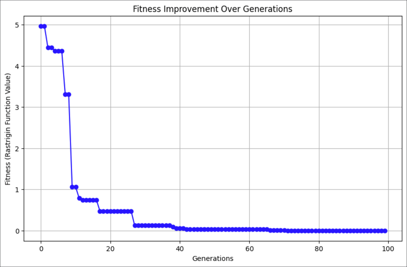
The graph above shows how the CSA found better solutions to the Rastrigin function with every generation.
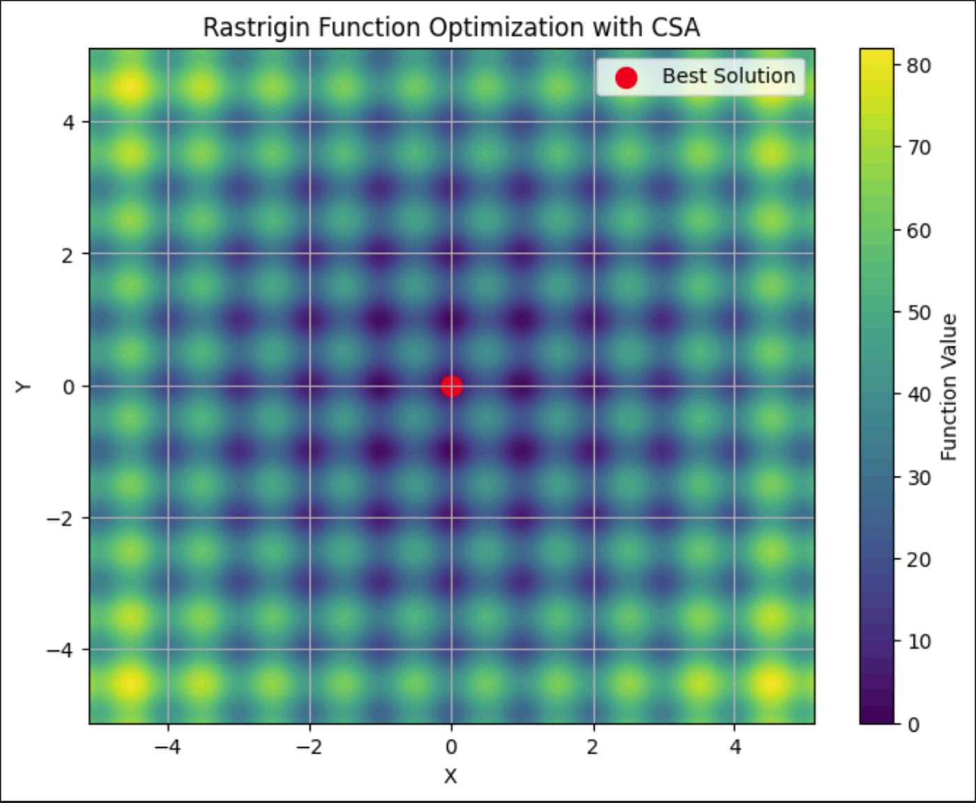
This graph shows the Rastrigin plotted, demonstrating it’s many local minima. The best solution, the red dot in the middle, is the final solution found by the CSA.
NSA is particularly useful for anomaly detection tasks. This algorithm simulates how the immune system distinguishes between the body’s own cells and foreign invaders. In an NSA, you generate a set of detectors that do not match the normal data patterns. These detectors are then used to monitor new data, flagging anything that appears anomalous.
Here’s an overview of how to create an NSA:
Let's see how this works using a fictional set of transactions. In this example, we generate normal transactions centered around two clusters and fraudulent transactions scattered randomly. We’ll employ a negative selection algorithm, where fraud detectors are scattered across the feature space to identify anomalies based on their proximity to these detectors.
import numpy as np
import matplotlib.pyplot as plt

# Generate a synthetic dataset
np.random.seed()

# Parameters for bimodal distribution
num_normal_points = 80  # total number of normal transactions
num_points_per_cluster = num_normal_points // 2  # number of points in each cluster

# Generate normal transactions for two clusters
cluster1_center = [2, 2]
cluster2_center = [8, 8]

# Generate points around the first cluster center
normal_cluster1 = np.random.normal(loc=cluster1_center, scale=0.5, size=(num_points_per_cluster, 2))

# Generate points around the second cluster center
normal_cluster2 = np.random.normal(loc=cluster2_center, scale=0.5, size=(num_points_per_cluster, 2))

# Combine clusters into one dataset
normal_transactions = np.vstack([normal_cluster1, normal_cluster2])

# Define random distribution for fraudulent transactions
num_fraud_points = 5  # number of fraudulent transactions
fraudulent_transactions = np.random.uniform(low=0, high=10, size=(num_fraud_points, 2))

# Combine into one dataset
data = np.vstack([normal_transactions, fraudulent_transactions])
labels = np.array([0] * len(normal_transactions) + [1] * len(fraudulent_transactions))

# Function to generate detectors (random points) that don't match any of the normal data
def generate_detectors(normal_data, num_detectors, detector_size):
    detectors = []
    while len(detectors) < num_detectors:
        detector = np.random.rand(detector_size) * 10  # Scale to cover the data range
        if not any(np.allclose(detector, pattern, atol=0.5) for pattern in normal_data):
            detectors.append(detector)
    return np.array(detectors)

# Function to detect anomalies (points in the data that are close to any detector)
def detect_anomalies(detectors, data, threshold=0.5):
    anomalies = []
    for point in data:
        if any(np.linalg.norm(detector - point) < threshold for detector in detectors):
            anomalies.append(point)
    return anomalies

# Generate detectors that do not match the normal data
detectors = generate_detectors(normal_transactions, num_detectors=300, detector_size=2)

# Detect anomalies within the entire dataset using the detectors
anomalies = detect_anomalies(detectors, data)
print("Number of anomalies detected:", len(anomalies))

# Convert anomalies to a numpy array for visualization
anomalies = np.array(anomalies) if anomalies else np.array([])

# Define axis limits
x_min, x_max = 0, 10
y_min, y_max = -1, 11

# Visualize the dataset, detectors, and anomalies
plt.figure(figsize=(14, 6))

# Plot the normal transactions and fraudulent transactions
plt.subplot(1, 2, 1)
plt.scatter(normal_transactions[:, 0], normal_transactions[:, 1], color='red', marker='x', label='Normal Transactions')
plt.scatter(fraudulent_transactions[:, 0], fraudulent_transactions[:, 1], color='green', marker='o', label='Fraudulent Transactions')
plt.scatter(detectors[:, 0], detectors[:, 1], color='blue', marker='o', alpha=0.5, label='Detectors')
if len(anomalies) > 0:
    plt.scatter(anomalies[:, 0], anomalies[:, 1], color='yellow', marker='*', s=100, label='Detected Anomalies')
plt.xlabel('Feature 1')
plt.ylabel('Feature 2')
plt.title('Fraud Detection Using Negative Selection Algorithm (NSA)')
plt.legend(loc='lower right')
plt.xlim(x_min, x_max)
plt.ylim(y_min, y_max)
plt.grid(False)

# Create a grid of points to classify
xx, yy = np.meshgrid(np.linspace(x_min, x_max, 100), np.linspace(y_min, y_max, 100))
grid_points = np.c_[xx.ravel(), yy.ravel()]

# Classify grid points
decision = np.array([any(np.linalg.norm(detector - point) < 0.5 for detector in detectors) for point in grid_points])
decision = decision.reshape(xx.shape)

# Plot the decision boundary
plt.subplot(1, 2, 2)
plt.contourf(xx, yy, decision, cmap='coolwarm', alpha=0.3)
plt.scatter(normal_transactions[:, 0], normal_transactions[:, 1], color='red', marker='x', label='Normal Transactions')
plt.scatter(fraudulent_transactions[:, 0], fraudulent_transactions[:, 1], color='green', marker='o', label='Fraudulent Transactions')
plt.scatter(detectors[:, 0], detectors[:, 1], color='blue', marker='o', alpha=0.5, label='Detectors')
if len(anomalies) > 0:
    plt.scatter(anomalies[:, 0], anomalies[:, 1], color='yellow', marker='*', s=100, label='Detected Anomalies')
plt.xlabel('Feature 1')
plt.ylabel('Feature 2')
plt.title('Decision Boundary Visualization')
plt.legend(loc='lower right')
plt.xlim(x_min, x_max)
plt.ylim(y_min, y_max)
plt.grid(False)

# Show the plot
plt.show()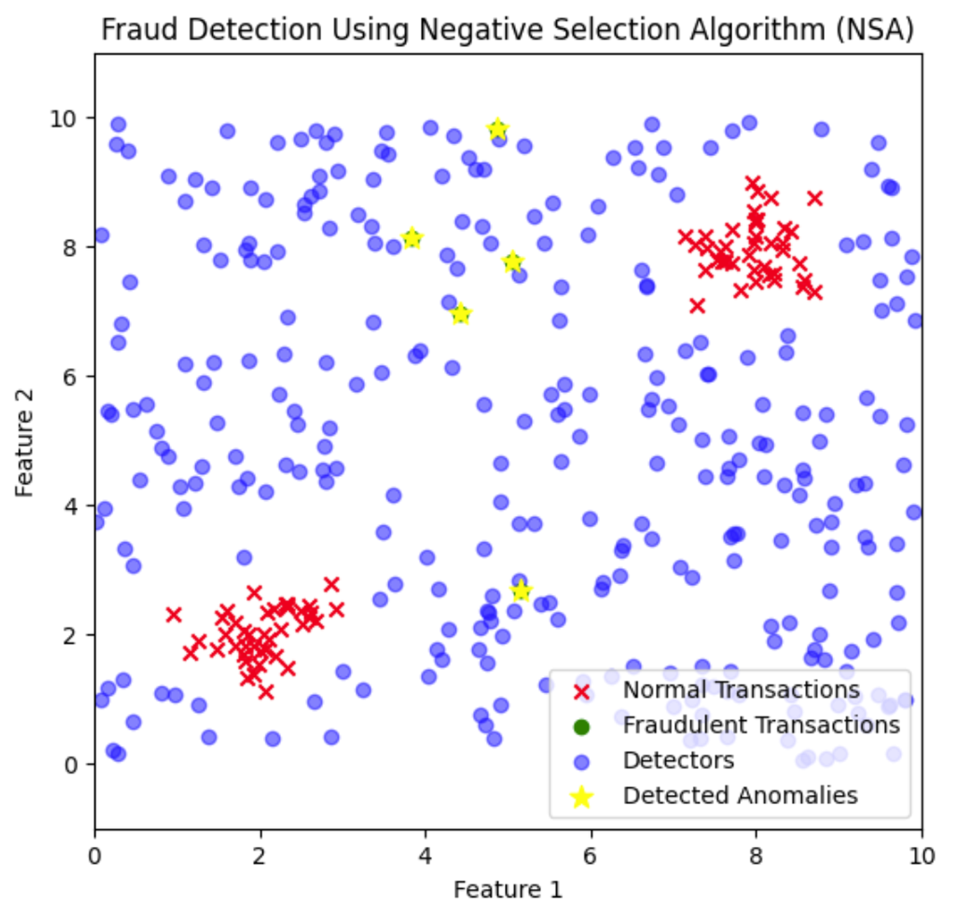
Here, the fraud detectors are distributed across the feature space to cover areas where normal transactions do not appear. Fraudulent transactions that fall close to these detectors are identified and flagged as anomalies.
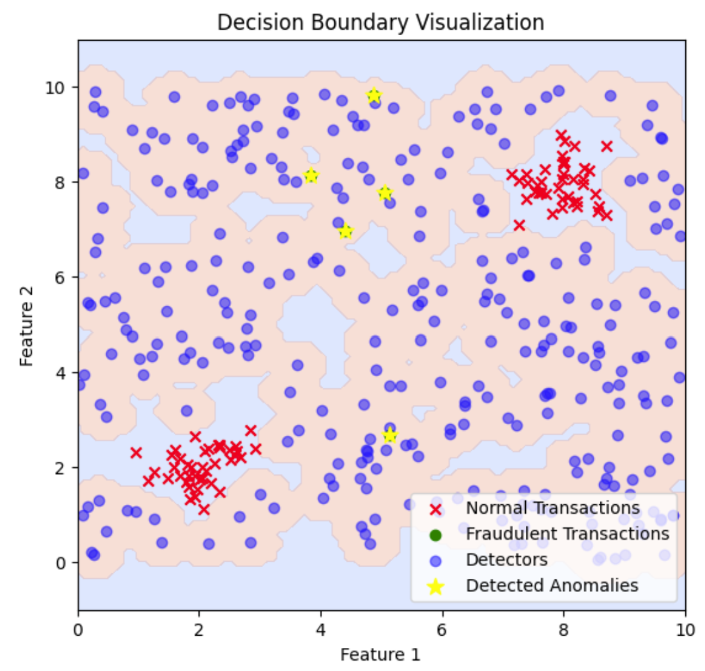
This plot illustrates the decision boundary created by the fraud detectors. The shaded regions represent areas classified as anomalous based on the proximity to the detectors, highlighting where fraudulent transactions are detected in relation to normal transactions. To adjust the decision boundary and cover more or less area, you can modify the distance threshold used for detecting anomalies, which will expand or contract the regions classified as anomalous.
INT is inspired by the idea that immune responses are not only based on individual antibodies but also on their communication. This approach models the immune system as a network where antibodies communicate to enhance the overall immune response. In this context, each antibody (solution) can interact with others to influence and refine the search for optimal solutions.
Here’s how you can implement a basic version of INT in Python:
Let's use INT to predict stock market trends based on a set of economic indicators. We'll use a fictional dataset where each solution represents a combination of indicators for forecasting stock prices.
import numpy as np
import matplotlib.pyplot as plt
from sklearn.linear_model import LinearRegression
from sklearn.metrics import mean_squared_error

# Generate synthetic data for illustration
np.random.seed(42)
n_samples = 100
n_features = 5
X = np.random.rand(n_samples, n_features)  # Random economic indicators
true_weights = np.array([0.5, -0.2, 0.3, 0.1, -0.1])
y = X @ true_weights + np.random.normal(0, 0.1, n_samples)  # Stock prices with noise

# Define the fitness function
def fitness_function(solution, X, y):
    model = LinearRegression()
    model.coef_ = solution
    predictions = X @ model.coef_
    return mean_squared_error(y, predictions)

# Generate the initial population of potential solutions
def generate_initial_population(pop_size, solution_size):
    return np.random.uniform(-1, 1, size=(pop_size, solution_size))

# Create the immune network
def create_immune_network(population, fitness, num_neighbors):
    network = []
    for i, individual in enumerate(population):
        distances = np.linalg.norm(population - individual, axis=1)
        neighbors = np.argsort(distances)[1:num_neighbors+1]  # Exclude self
        network.append(neighbors)
    return network

# Update the immune network
def update_network(network, population, fitness, mutation_rate):
    new_population = np.copy(population)
    for i, neighbors in enumerate(network):
        if np.random.rand() < mutation_rate:
            # Apply mutation with a smaller range
            mutation = np.random.uniform(-0.05, 0.05, population.shape[1])
            new_population[i] += mutation
    return new_population

# Main function implementing Immune Network Theory
def immune_network_theory(solution_size=n_features, pop_size=50, num_neighbors=5, mutation_rate=0.1, generations=50):
    population = generate_initial_population(pop_size, solution_size)
    best_fitness_per_generation = []  # Track the best fitness in each generation

    for generation in range(generations):
        fitness = np.array([fitness_function(ind, X, y) for ind in population])
        network = create_immune_network(population, fitness, num_neighbors)
        new_population = update_network(network, population, fitness, mutation_rate)

        # Evaluate the fitness of the new population
        fitness_new = np.array([fitness_function(ind, X, y) for ind in new_population])

        # Combine the old and new populations
        combined_population = np.vstack((population, new_population))
        combined_fitness = np.hstack((fitness, fitness_new))

        # Select the best individuals
        best_indices = np.argsort(combined_fitness)[:pop_size]
        population = combined_population[best_indices]
        fitness = combined_fitness[best_indices]

        # Track the best fitness of this generation
        best_fitness = np.min(fitness)
        best_fitness_per_generation.append(best_fitness)

        # Stop early if the fitness is good enough
        if best_fitness < 0.01:
            print(f"Optimal solution found in {generation + 1} generations.")
            break

    # Plot the fitness improvement over generations
    plt.figure(figsize=(10, 6))
    plt.plot(best_fitness_per_generation, marker='o', color='blue', label='Best Fitness per Generation')
    plt.xlabel('Generations')
    plt.ylabel('Mean Squared Error')
    plt.title('Fitness Improvement Over Generations')
    plt.grid(True)
    plt.show()

    # Return the best solution found
    best_solution = population[np.argmin(fitness)]
    return best_solution

# Example Usage
best_solution = immune_network_theory()
print("Best solution found (economic indicators weights):", best_solution)
print("Mean Squared Error at best solution:", fitness_function(best_solution, X, y))

# Plot the predicted vs. actual values using the best solution
model = LinearRegression()
model.coef_ = best_solution
predictions = X @ model.coef_

plt.figure(figsize=(8, 6))
plt.scatter(y, predictions, c='blue', label='Predicted vs Actual')
plt.plot([min(y), max(y)], [min(y), max(y)], 'r--', label='Ideal Fit')
plt.xlabel('Actual Values')
plt.ylabel('Predicted Values')
plt.title('Stock Price Prediction with INT')
plt.legend()
plt.grid(True)
plt.show()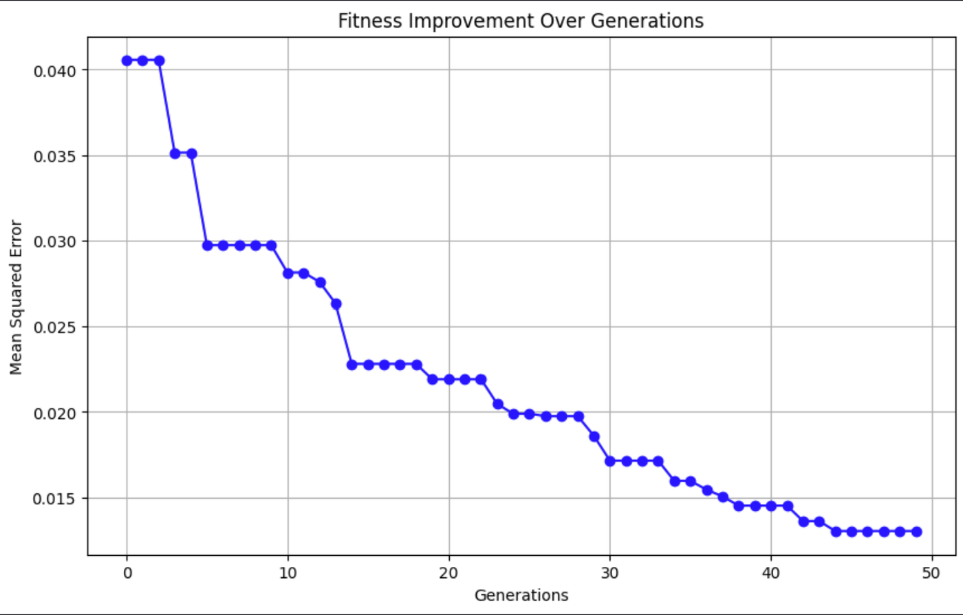
This graph shows the Mean Squared Error (MSE) decreasing over time, indicating that the model's predictions are getting more accurate.
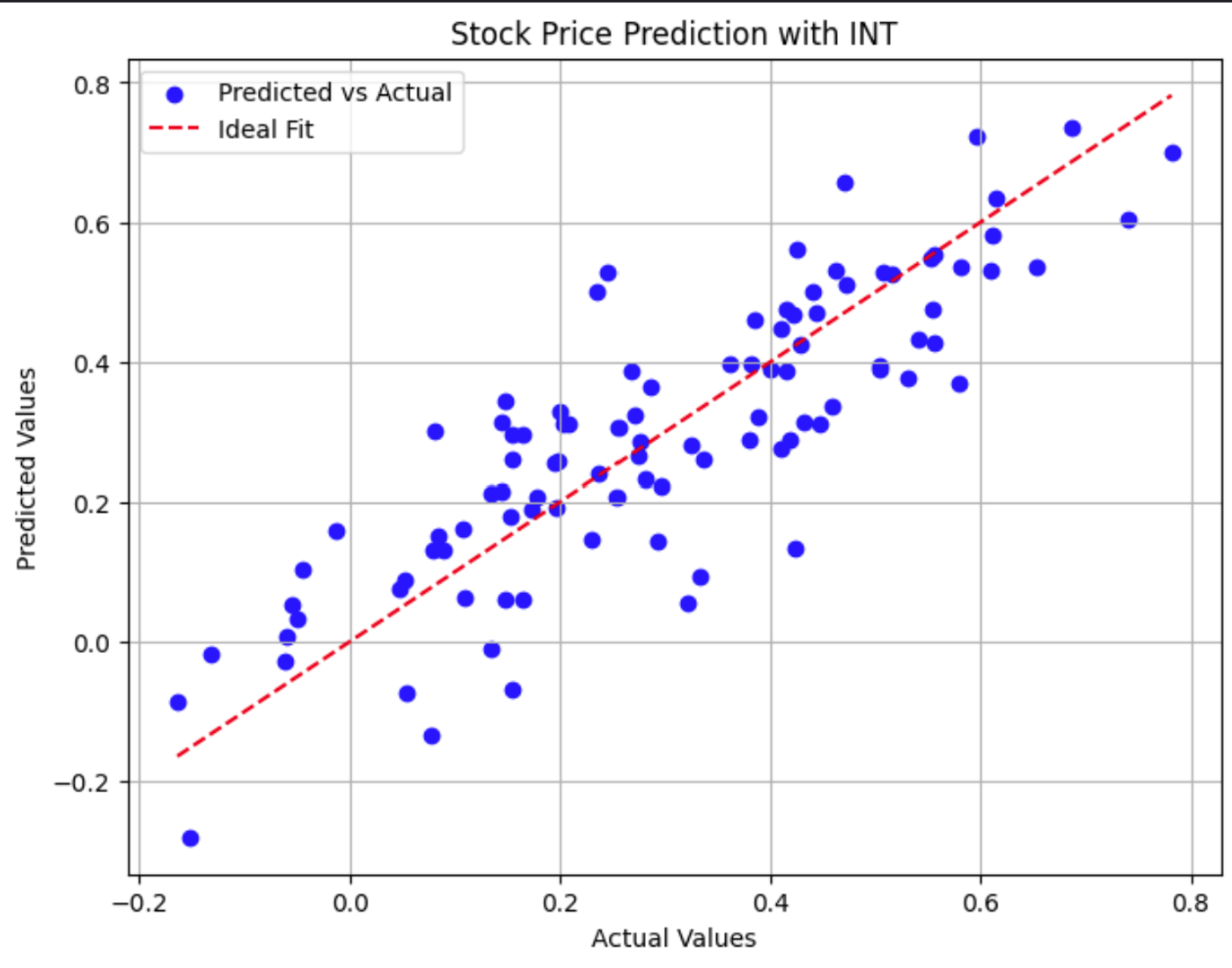
This scatter plot compares actual stock prices to model predictions. Points closer to the red dashed line show more accurate predictions.
AIS is one of many machine learning techniques that draws inspiration from biology.
Neural networks are inspired by the human brain and excel at learning from large datasets. They are used for tasks like image recognition and natural language processing. They rely on extensive training with vast amounts of data to adjust interconnected neurons’ weights.
In contrast, artificial immune systems focus on adaptability and decentralized problem-solving without requiring large datasets. AIS mimic the immune system's ability to recognize and respond to new challenges in real-time, making them suitable for dynamic environments where rapid adaptation is crucial.
Genetic algorithms, inspired by natural evolution, are effective for optimizing complex problems by evolving a population of solutions through selection, crossover, and mutation. This process is similar to CSA.
However, while genetic algorithms rely on genetic operators to explore the solution space, CSA adapts solutions by mimicking immune responses, offering flexibility in dealing with new and unexpected challenges. AIS, including CSA, are particularly effective in dynamic environments where rapid adaptation and continuous learning are crucial.
You can read more about genetic algorithms in Genetic Algorithm: Complete Guide With Python Implementation.
Swarm intelligence algorithms are inspired by the collective behavior of social organisms like ants and bees. They use decentralized systems and simple agent interactions to achieve complex global optimization.
This is similar, in spirit, to INT. Both approaches focus on maintaining diversity and adaptability within a system to address optimization problems. While swarm intelligence emphasizes agent-based interactions, INT leverages mechanisms akin to immune responses, offering complementary methods for dynamic problem-solving.
You can read more about swarm intelligence algorithms in Swarm Intelligence Algorithms: Three Python Implementations.
Artificial immune systems hold promise for solving complex problems across various domains. Researchers are working to enhance these systems to make them even more useful.
One area researchers are exploring is how to create hybrid models that combine AIS with other computational intelligence techniques. The hope is that these hybrid models will be more robust and versatile.
These hybrid approaches aim to use the strengths of each method, such as AIS's adaptive capabilities and neural networks' powerful learning mechanisms. For more information, check out Artificial Immune Systems.
Another active research area involves applying AIS to new domains. While traditionally used in cybersecurity and optimization, AIS is now being explored in fields like robotics, bioinformatics, and even financial modeling. The adaptability and decentralized nature of AIS make it a promising candidate for solving problems in these dynamic and often unpredictable environments. For more information, I encourage you to read Nature-Inspired Computing: Scope and Applications of Artificial Immune Systems Toward Analysis and Diagnosis of Complex Problems.
AIS models not only offer enhanced computational techniques but can also contribute to our understanding of real immune systems. They are advancing immunotherapy strategies for diseases such as cancer and autoimmune disorders. Check out this collaboration between the Cleveland Clinic and IBM to learn more.
Artificial immune systems offer a unique approach to solving complex problems by drawing inspiration from the human immune system. By emulating biological processes like pattern recognition, adaptation, and memory, AIS provide versatile solutions in fields ranging from cybersecurity to optimization.
Learn how to work with LLMs in Python right in your browser
Learn AI with these courses!
Track
Track
Course
blog
Armstrong Asenavi
15 min
blog
Matt Crabtree
11 min
cheat-sheet
Karlijn Willems
Tutorial
Rajesh Kumar
Tutorial
Bex Tuychiev
Tutorial
Amberle McKee