AutoSum in Excel: Add Numbers Instantly with One Click

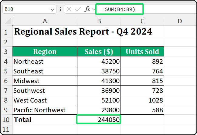
Adding numbers in Excel should be fast. You shouldn't have to type, for example, =SUM(B2:B47) every time you need a total. AutoSum does this automatically. One click, and Excel figures out what you want to add.

This tutorial walks you through everything AutoSum can do. I'll show you where to find it, how the shortcuts work on Windows and Mac, and what to do when it doesn't behave as expected. By the end, you'll use AutoSum without thinking about it.

How to Use AutoSum in Excel

AutoSum is straightforward once you understand its logic. Let me break down exactly how it works and where things can go wrong.

Where to find AutoSum in Excel

AutoSum lives in two places on the ribbon. On the Home tab, look for the Editing group on the far right. You'll see the Greek letter Sigma (Σ) with a small dropdown arrow. This is AutoSum.

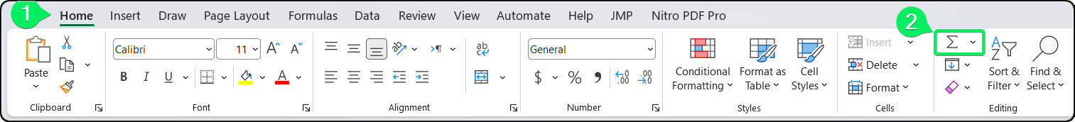
AutoSum button in the Home tab Editing group. Image by Author.

On the Formulas tab, AutoSum appears in the Function Library group near the left side. Same button, same functionality. I use the Home tab location because it's where I spend most of my time anyway.

The dropdown arrow reveals additional functions beyond Sum: Average, Count Numbers, Max, and Min. Clicking the Sigma icon directly inserts a SUM() formula. Clicking the arrow lets you choose a different calculation.

How AutoSum selects a range

Here's where AutoSum gets interesting. When you click the button, Excel doesn't just insert =SUM() and leave you to fill in the blanks. It analyzes your spreadsheet to guess which cells you want to add.

The algorithm follows a strict priority: check above first, then check left. If there are numbers directly above your cursor, AutoSum creates a vertical sum. If the cell above is empty or contains text, it pivots to check the cells to your left and creates a horizontal sum.

This happens instantly. You'll see a "marching ants" border around the proposed range. If the selection looks correct, press Enter. If not, drag to adjust before confirming.

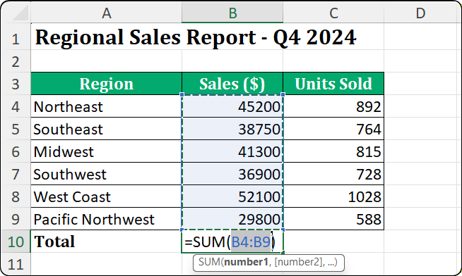
Marching ants show the detected range. Image by Author.

The detection stops at boundaries. A blank cell, a text label, or the edge of the worksheet all signal "stop here." This is usually helpful because it excludes headers automatically. But it can cause problems if your data has accidental gaps, which I'll cover in the troubleshooting section.

Using AutoSum for columns and rows

For column sums, position your cursor in the empty cell directly below your data. Click AutoSum. Excel proposes a range from the first number above to the cell just before your cursor.

Column sum appears below the last data row. Image by Author.

For row sums, position your cursor in the empty cell immediately to the right of your data. Click AutoSum. Excel scans leftward and proposes a horizontal range.

The key is cursor placement. AutoSum can only look up and left. It cannot detect data below or to the right of where you're sitting. If you click AutoSum in the wrong cell, you'll get unexpected results.

Using AutoSum across multiple ranges

AutoSum supports batch processing. Select multiple empty cells at once, then click AutoSum. Excel generates separate formulas for each cell simultaneously.

Here's a practical example. You have sales data in columns B, C, and D. You want totals for all three columns. Select B10:D10 (the row beneath all three columns), click AutoSum once, and Excel writes three SUM() formulas, one for each column.

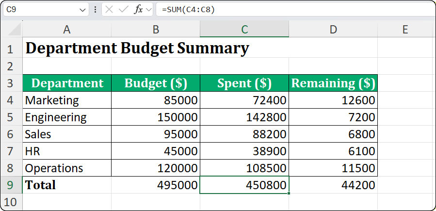
Batch processing three columns at once. Image by Author.

You can even do cross-footing. Select a block of data plus one empty row below and one empty column to the right. AutoSum calculates column totals in the bottom row and row totals in the right column, all in one click. This is a time saver for financial statements where you need both dimensions totaled.

AutoSum Shortcut in Excel

Mouse clicks are fine, but shortcuts are faster. If you're summing data frequently, memorize the keyboard shortcut for your platform.

Using the AutoSum keyboard shortcut

On Windows, the shortcut is Alt + = (hold Alt, press the equals sign). This triggers AutoSum instantly without touching the ribbon.

The shortcut works in two steps. The first press enters "point mode." Excel types =SUM(, guesses the range, and highlights it with marching ants. If the range looks correct, press Enter to confirm. If you want to accept quickly, press Alt + = again instead of Enter.

I use this shortcut constantly. Select a cell below your data, Alt + =, Enter. Three keystrokes and the sum is done.

Notes on platform differences

Mac users have a different shortcut: ⌘ + Shift + T (Command + Shift + T). This is a three-key combination, not two like Windows.

A common mistake: Mac users try Option + = expecting it to mirror the Windows Alt key. It doesn't work. Option + = often inserts a special character (≠) depending on your keyboard layout. Stick with ⌘ + Shift + T.

If you need Windows-style shortcuts on Mac, you can create a custom shortcut in macOS System Settings under Keyboard > Shortcuts > App Shortcuts. Map the menu command "AutoSum" to whatever key combination you prefer.

Using AutoSum for Average, Count, Max, and Min

AutoSum isn't limited to addition. The dropdown menu provides quick access to four other common aggregations.

Choosing other functions from AutoSum

Click the dropdown arrow next to the AutoSum button. You'll see five options: Sum, Average, Count Numbers, Max, and Min. Select one, and Excel inserts that function with the same intelligent range detection.

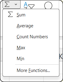
Five functions available from one button. Image by Author.

Average calculates the arithmetic mean of the selected range. I use this for performance scores, test results, and any dataset where the central tendency matters.

Max and Min find the largest and smallest values. These are useful for identifying outliers or setting benchmarks. "What was our best sales day?" Click Max. "What was our worst?" Click Min.

Count Numbers tallies how many cells contain numeric values. This is where things get nuanced.

Understanding differences between count options

The AutoSum menu says "Count Numbers," not just "Count." This matters. The underlying function is COUNT(), which only counts cells containing numbers, dates, or numeric formulas.

COUNT() ignores text, logical values (TRUE/FALSE), and errors. If you have a column of employee names and click Count Numbers, the result is zero. The names are text, not numbers.

If you need to count all non-empty cells regardless of content, use COUNTA() instead. AutoSum doesn't offer this directly, but you can type =COUNTA(range) manually or access it through More Functions in the dropdown.

AutoSum Not Working in Excel

When AutoSum fails, the cause is almost never a bug. It's usually a data issue you can fix once you know what to look for.

Numbers stored as text

This is the most common AutoSum failure. Your cells look like numbers, but Excel treats them as text. The SUM() formula ignores them, returning zero or an incomplete total.

How do you identify this? Look for these clues: the numbers align left instead of right (numbers default to right alignment), there's a small green triangle in the cell's top-left corner, or the status bar shows only COUNT when you select the range (not SUM or AVERAGE).

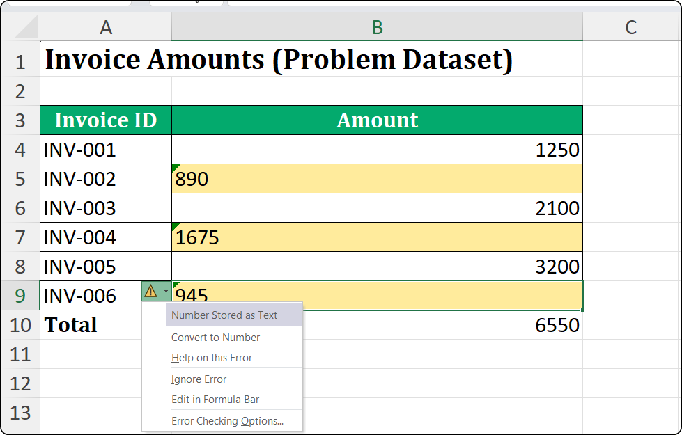
Green triangles indicate numbers stored as text. Image by Author.

This happens frequently with data imported from CSV files, databases, banking systems, or web pages. These sources often format numbers as text to preserve leading zeros or special characters.

There are several fixes. The fastest for small ranges: click the yellow warning icon that appears next to the green triangle and select Convert to Number. For large datasets, select the column, go to Data > Text to Columns, and click Finish immediately without changing any settings. This forces Excel to re-evaluate data types.

Another trick I use: type the number 1 in an empty cell, copy it, select your problematic data, and use Paste Special > Multiply. This mathematical operation coerces text to numbers without changing values.

Incorrect range selection

Sometimes AutoSum selects fewer cells than you expect. This usually happens because of blank cells in your data. If row 10 in your column is empty, and you trigger AutoSum from row 20, Excel only captures rows 11-19. The data in rows 2-9 is silently excluded.

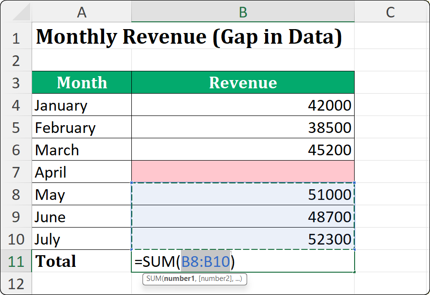
Gap in data breaks range detection. Image by Author.

The fix is prevention: keep your data contiguous. If blanks are unavoidable, fill them with zeros. Alternatively, manually adjust the range after AutoSum proposes its guess. Just drag the marching ants border to include all your data. This visual check takes one second and prevents errors that can take hours to find later.

Issues with merged cells

Merged cells break AutoSum's logic. When you merge cells, only the top-left cell actually contains data. The other cells in the merge become effectively empty, even if they appear to span content.

AutoSum may select unexpected ranges when it encounters merged cells. The cursor might seem to jump unpredictably, or the formula might include cells you didn't intend.

My advice: avoid merging cells in data ranges entirely. If you need a centered header that spans multiple columns, use Format Cells > Alignment > Center Across Selection instead. This creates the visual effect of merging without combining the underlying cells, keeping your calculations intact.

AutoSum with Filtered Data in Excel

When you filter data, AutoSum's behavior depends on which function underlies the calculation. This catches many users off guard.

How AutoSum handles filtered rows

By default, AutoSum inserts the SUM() function. Here's the critical point: SUM includes all cells in the range, whether visible or not. The formula =SUM(A2:A100) always adds A2 through A100, regardless of which rows are hidden.

This seems wrong until you understand the logic. SUM calculates based on cell addresses, not visibility. The formula =SUM(A2:A100) always adds A2 through A100, regardless of which rows are hidden.

When you need a total that respects filters, you need SUBTOTAL(). The good news: if you apply a filter first and then click AutoSum, Excel automatically inserts SUBTOTAL instead of SUM. It knows you probably want filtered-aware calculations.

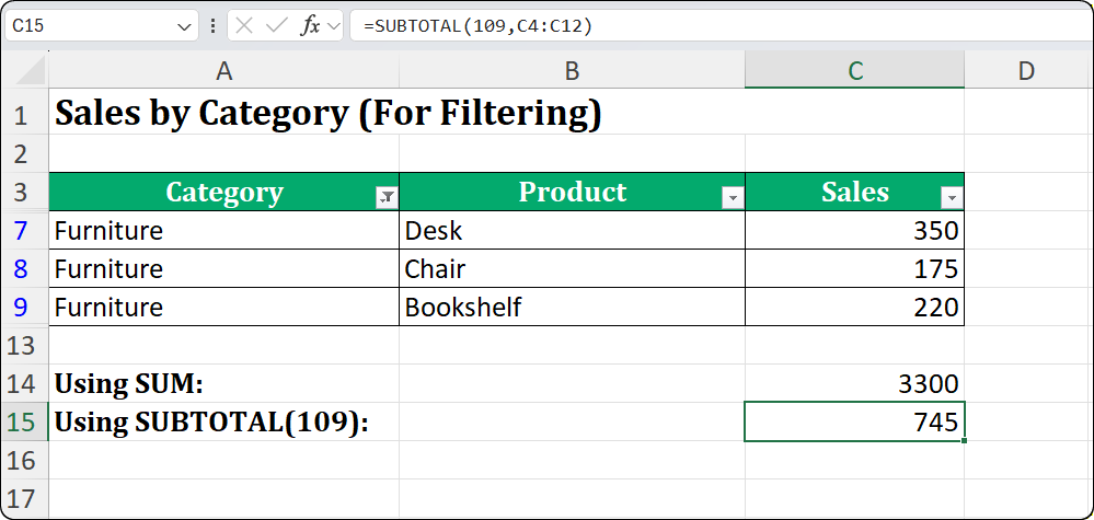
SUBTOTAL() respects filtered row visibility. Image by Author.

Understanding subtotal arguments

SUBTOTAL() offers two argument options. SUBTOTAL(9, range) excludes filtered rows but includes manually hidden rows. SUBTOTAL(109, range) excludes both filtered and manually hidden rows.

For most users, the distinction doesn't matter. But if you're building dashboards where users might filter or manually hide rows, use SUBTOTAL(109, range) for the most intuitive behavior. The total always matches exactly what's visible on screen.

Excel Tables handle this automatically. When you convert data to a Table (Ctrl + T) and enable the Total Row, Excel uses SUBTOTAL(109) by default. It's one of many reasons I recommend Tables for any dataset that will be filtered regularly. If you want to learn more about dynamic data handling, our Data Analysis in Excel course covers Tables in depth.

Best Practices for Using AutoSum Reliably

After years of building financial models and cleaning messy datasets, I've developed habits that prevent AutoSum headaches. Here's what works.

• Keep data contiguous. No blank rows or columns in the middle of your data. If you need visual separation, use borders or cell shading, not empty rows.

• Use one header row with text labels. If your header contains a number (like a year "2024"), Excel might include it in calculations. Keep headers clearly textual.

• Avoid merged cells in calculation areas. Use "Center Across Selection" for visual spanning.

• Verify the selected range every time. If AutoSum stopped short or went too far, you'll catch it immediately. This habit has saved me countless debugging sessions.

• Convert data to Excel Tables for growing datasets. Tables expand automatically when you add rows. The Total Row uses SUBTOTAL(109) and always stays attached to the data. You'll never have a sum formula that misses new entries.

• Prefer AutoSum for quick totals, manual formulas for complex logic. AutoSum excels at straightforward sums, averages, and counts. If you need conditional logic, multiple criteria, or references to non-adjacent ranges, write the formula yourself. Use SUMIF() or SUMIFS() for conditional summing, and AGGREGATE() when you need error handling.

Conclusion

AutoSum is deceptively simple. Click a button, get a total. But understanding the logic underneath (the up-left priority, the boundary detection, the filtered data behavior) transforms it from a convenience feature into a reliable tool.

The shortcuts alone will save you hours over a year of spreadsheet work. Memorize them and use them without thinking.

When AutoSum misbehaves, you now know where to look: numbers stored as text, blank cells breaking ranges, or merged cells. These aren't bugs. They're data issues with straightforward fixes.

Start using AutoSum deliberately. Check your totals and build the habit of verification. When your data grows complex, consider converting to Excel Tables. They handle the edge cases automatically.

If you want to deepen your Excel skills, including formulas, data manipulation, and analysis techniques, explore our Excel fundamentals track. Your future self will thank you for the time invested.