Track
In this article, we will explore an important technique in statistics and machine learning called bootstrapping. Bootstrapping takes its name from the phrase, ‘pulling yourself up by your bootstraps,’ because the statistical technique of bootstrapping allows you to do so much with very little. With bootstrapping, you can take a distribution of any shape or size and create a new distribution of resamples, and use this new distribution to approximate the true probability distribution. For this reason, bootstrapping is an especially effective way of assigning measures of accuracy such as bias, variance, confidence intervals, and prediction error to sample estimates.
Before we get started, if you are interested in data science, consider taking these DataCamp courses on data science and statistics, such as our Statistical Inference in R skill track and our Foundations of Inference in Python course.
Bootstrapping and Other Resampling Methods
Let’s start by anchoring bootstrapping correctly in its place among resampling methods. Although there are different kinds of resampling methods, they share one important thing in common: they mimic the sampling process. The reason we use a resampling method is because it isn’t practical to keep taking new samples from our population of interest, and resampling is a sort of shortcut.
For example, when we want to understand something about our population of interest, we may consider running a survey and hoping for one thousand responses. However, no one will administer the same survey into a target population one thousand times. It is because of this practical limitation that we use a resampling method in order to generate statistics about our sample, such as the standard error.
Types of resampling methods
There are four main types of resampling methods. It’s worth mentioning the other resampling methods because they share a common history of statistical innovation and improvement. In particular, bootstrapping has been developed as an extension or modification or improvement upon the jackknife method.
- Permutation Resampling: Also known as randomization or shuffling, this method involves randomly rearranging the data to test hypotheses by comparing observed results to what might occur under a null hypothesis.
- Jackknife Resampling: In jackknife resampling, each observation is systematically left out of the sample one at a time, and the statistic is recalculated. This method is used to estimate the bias and variance of a statistical estimator.
- Bootstrap Resampling: This method involves randomly sampling with replacement from the original dataset to create multiple smaller samples. It is commonly used to estimate the distribution of a statistic.
- Cross-Validation: Cross-validation divides the data into subsets, or folds, and trains the model on some while testing it on others. This helps to assess the model's performance on unseen data and prevent overfitting.
The jackknife vs. the bootstrap method
It’s useful in particular to talk a bit about the jackknife because the jackknife is a precursor to bootstrapping, and bootstrapping was introduced as a sort of extension and improvement on the jackknife, which was developed in the 1950s when computers had about one kilobyte of memory.
The jackknife is a leave-one-out resampling method that calculates a statistic of interest; it does this successively or iteratively until each observation has been removed. With the jackknife, the number of resamples is limited to the number of observations, and largely for this reason, the jackknife performs a little bit poorly with small sample sizes. Jackknife is also a little bit limited in terms of the kinds of data that can be used. On the other hand, unlike the bootstrap, the jackknife is reproducible every time.
Applications of Bootstrapping
Bootstrapping has a wide range of applications in both statistics and machine learning. One of its most common uses is to estimate confidence intervals when the underlying distribution is unknown or when sample sizes are small. This capability makes bootstrapping particularly valuable in situations where traditional parametric methods might not be appropriate.
Also, bootstrapping is often used in hypothesis testing and model validation, where it can help evaluate the robustness of a model’s predictions. In machine learning, bootstrapping underpins the popular ensemble method known as bagging, which is used in models like random forests to improve accuracy by reducing variance.
How to Do Bootstrap Resampling
To illustrate bootstrapping, we need to use a programming language like R because it allows us to generate multiple resampled datasets; without a programming environment, the process would be too time-consuming and complex to perform manually. For this article, we will consider how to bootstrap the confidence intervals for a distribution and also for a linear regression using the Fish Market dataset on Kaggle.
Sampling with and without replacement
Before looking at bootstrapping properly, it’s useful to first get familiar with the idea of sampling with replacement. Here, the base R sample() function takes at least two arguments that need to be explicitly decided in the function call: x, and size. x decides the list or range of values from which we are choosing to make a sample and size decides the size of our sample. There is an additional argument that is often explicitly specified, which is the replace argument. Unless otherwise decided, replace = FALSE is set as the default.
Bootstrapping is sampling with replacement. When we sample with replacement, we are replacing the value after every sample. Each sample is, therefore, independent of the value that came before it. When we sample without replacement, we aren’t replacing values, so once a value is selected, it cannot be selected again, so we can say that the two sample values are not independent, and whatever value we get on one sample affects the possibility of the values from the next sample. A consequence here is that we cannot choose a sample size larger than the size of the input vector unless we specify replace = TRUE. Bootstrapping doesn't run into this issue, and we can generate a bootstrapped resampled dataset that is much larger than our original.
sample_without_replacement <- sample(x = 1:10, size = 10) # replace = FALSE as defaultsample_with_replacement <- sample(x = 1:10, size = 10, replace = TRUE)sample_with_replacement_and_weighted_probability <- sample(x = c(1, 0), size = 10, replace = TRUE, prob = c(0.8, 0.2))Bootstrapping confidence intervals for a distribution
Let’s now download our dataset and read it from our downloads folder into RStudio using the read.csv() function.
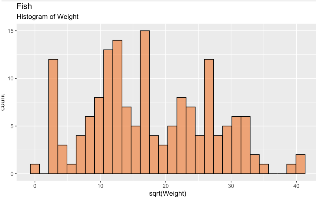
fish_df <- read.csv('~/Downloads/FISH.csv')To start, let's first create a histogram of the square root of fish weight, in order to see our distribution. This distribution, as we can see, is far from a normal, or Gaussian distribution. If anything, it is somewhat bimodal.
fish_df <- fish_df %>% mutate(sqrt_Weight = sqrt(Weight))ggplot(fish_df, aes(x = sqrt(Weight))) + geom_histogram(color = 'black', fill = '#ef8a47', alpha = 0.75) + labs(title = "Fish", subtitle = "Histogram of Weight")
Histogram of fish weight. Image by Author.
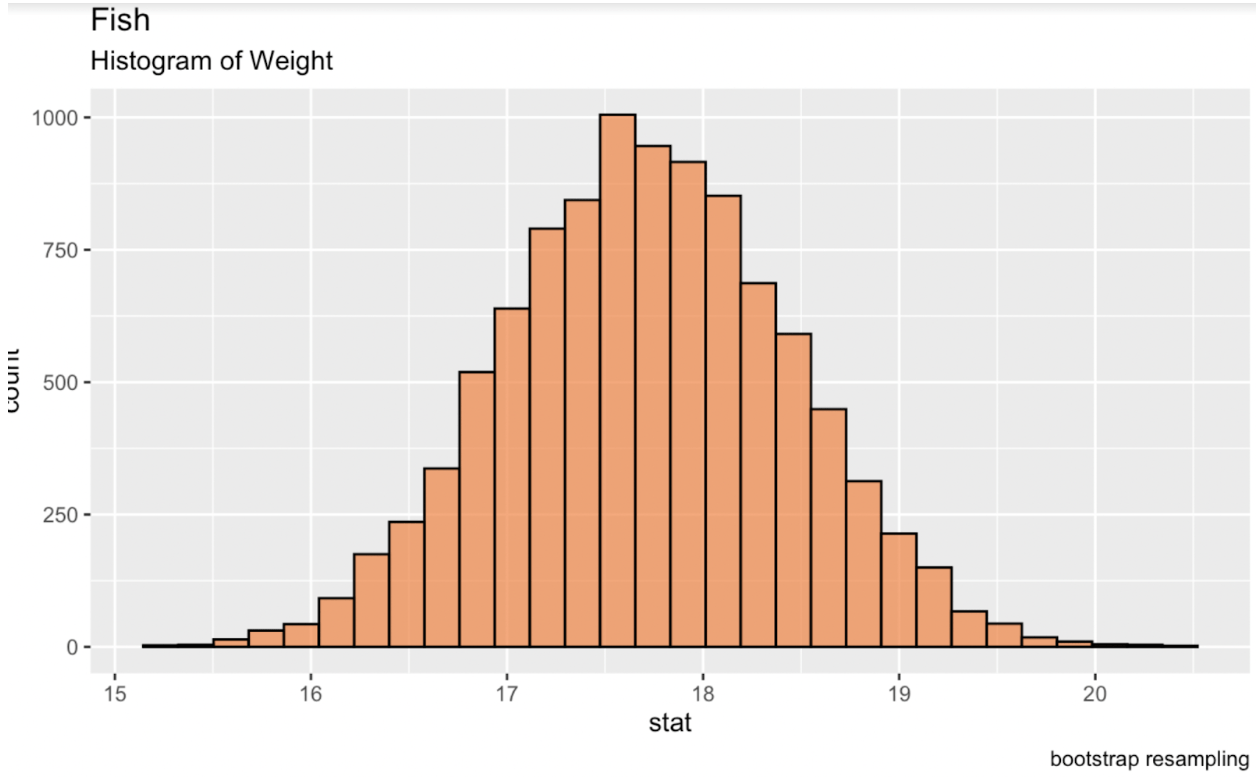
We can bootstrap in R by using the infer package from the tidymodels library. Printing this table to our console gives us a data frame of the desired statistic for each replicate. When we create a new distribution of these replicates, this distribution will be a normal distribution from which we can generate confidence intervals.
library(tidymodels)fish_df %>% dplyr::select(sqrt_Weight) %>% specify(response = sqrt_Weight) %>% generate(reps = 10000, type = 'bootstrap') %>% calculate(stat = 'mean') -> fish_bootstrapped_ci_dfggplot(fish_bootstrapped_ci_df, aes(x = stat)) + geom_histogram(color = 'black', fill = '#ef8a47', alpha = 0.75) + labs(title = "Fish", subtitle = "Histogram of Weight") Histogram of the bootstrapped mean of fish weight. Image by Author.
Bootstrapping confidence intervals for regression
Linear regression, the cornerstone of statistical modeling, is used to show the relationship between one or more independent variables and a dependent variable. When working with regression models, it’s common to assess uncertainty around our estimates. One way to do this is by calculating linear regression confidence intervals, which provide a range of values within which the true parameter, such as the mean, is likely to fall. Here, we will create confidence intervals using bootstrapping, and we will also create confidence intervals using the normal approximation method, also called the Wald confidence interval.
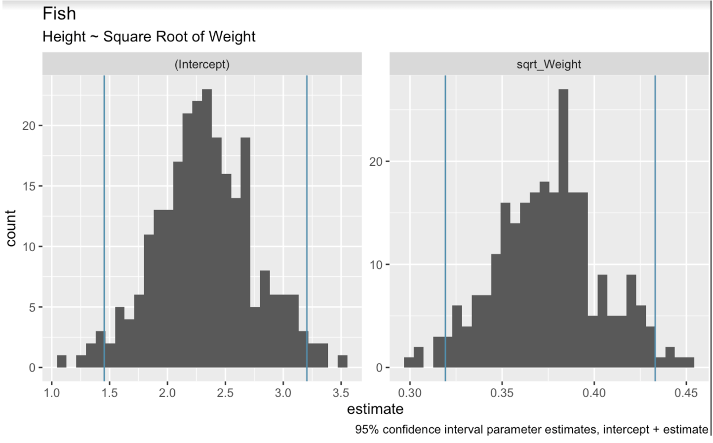
In the context of linear regression, bootstrap resampling involves randomly sampling from the dataset to create multiple bootstrap samples. We then fit a regression model to each sample. Finally, we use the distribution of model coefficients across these samples to estimate confidence intervals. In the following code, we use the bootstraps() function from the tidymodels package to perform bootstrap resampling on our dataset. We then create histograms to show the range of values that are present in our bootstrap resamples for the intercept and weight coefficients.
boots <- bootstraps(fish_df, times = 250, apparent = TRUE)fit_lm_on_bootstrap <- function(split) { lm(Height ~ sqrt_Weight, analysis(split))}boot_models <- boots %>% dplyr::mutate(model = map(splits, fit_lm_on_bootstrap), coef_info = map(model, tidy))boot_coefs <- boot_models %>% unnest(coef_info)percentile_intervals <- int_pctl(boot_models, coef_info)ggplot(boot_coefs, aes(estimate)) + geom_histogram(bins = 30) + facet_wrap( ~ term, scales = "free") + labs(title="fish", subtitle = "Height ~ Square Root of Weight") + labs(caption = "95% confidence interval parameter estimates, intercept + estimate") + geom_vline(aes(xintercept = .lower), data = percentile_intervals, col = '#528fad') + geom_vline(aes(xintercept = .upper), data = percentile_intervals, col = '#528fad')
Linear model bootstrapped coefficients. Image by Author.
When we graph our possible regression lines, we will clip the most extreme lines on either end in order to get a 95% interval. The int_pctl() function makes this easy.
boot_aug <- boot_models %>% sample_n(50) %>% mutate(augmented = map(model, augment)) %>% unnest(augmented)boots <- bootstraps(fish_df, times = 250, apparent = TRUE)fit_lm_on_bootstrap <- function(split) { lm(Height ~ sqrt_Weight, analysis(split))}boot_models <- boots %>% dplyr::mutate(model = map(splits, fit_lm_on_bootstrap), coef_info = map(model, tidy))boot_coefs <- boot_models %>% unnest(coef_info)percentile_intervals <- int_pctl(boot_models, coef_info)boot_aug <- boot_models %>% sample_n(50) %>% mutate(augmented = map(model, augment)) %>% unnest(augmented)As a final step, let’s now create confidence intervals that would be generated from the more theoretical, closed-form equations. We can find the parameters by calling summary() of our linear model object.
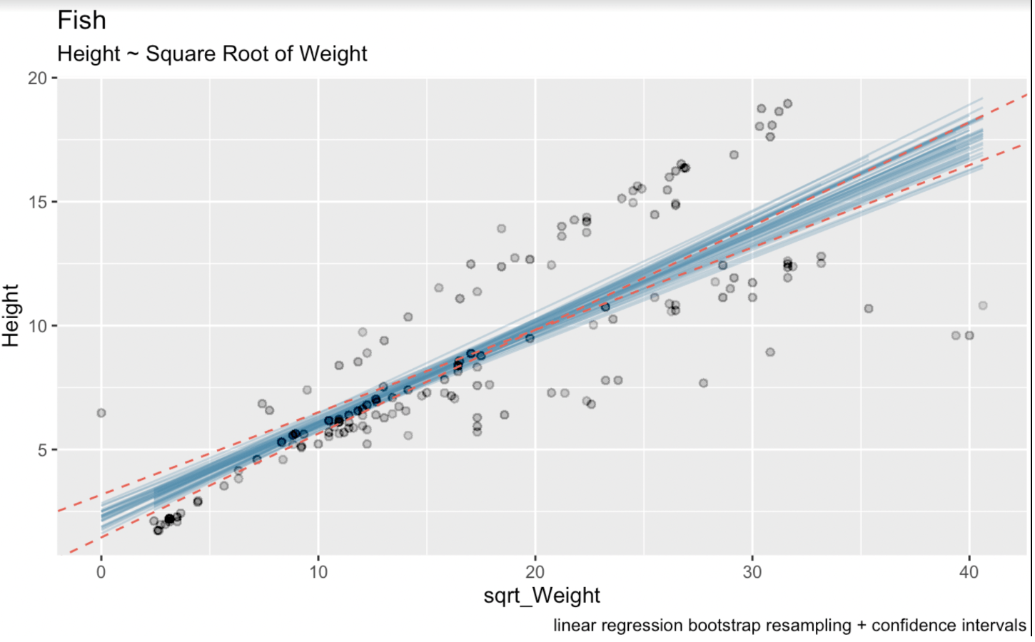
linear_model <- lm(Height ~ sqrt(Weight), fish_df)summary(linear_model)Call:lm(formula = Height ~ sqrt(Weight), data = fish_df)Residuals: Min 1Q Median 3Q Max-7.7425 -1.3611 -0.5628 2.2606 5.0131Coefficients: Estimate Std. Error t value Pr(>|t|)(Intercept) 2.31506 0.43636 5.305 3.77e-07 ***sqrt(Weight) 0.37569 0.02186 17.183 < 2e-16 ***---Signif. codes: 0 ‘***’ 0.001 ‘**’ 0.01 ‘*’ 0.05 ‘.’ 0.1 ‘ ’ 1Residual standard error: 2.533 on 157 degrees of freedomMultiple R-squared: 0.6529, Adjusted R-squared: 0.6506F-statistic: 295.3 on 1 and 157 DF, p-value: < 2.2e-16Here, the estimated coefficient for the sqrt_Weight variable is 0.37569. The standard error for sqrt_Weight is 0.02186. The degrees of freedom are 157 (which is 159 observations in our dataset minus two estimated parameters). And the t-value for a 95% confidence interval that is two-tailed is 1.975189. We know this final number through the qt() function: qt(0.975, 157). In the below visualization, the blue lines are the bootstrapped linear regression lines, and the dotted red lines are the confidence interval generated by the common analytical formula.
# Wald confidence interval(CI_upper <- 0.37569 + 1.975 * 0.02186)(CI_lower <- 0.37569 - 1.975 * 0.02186)(CI_intercept_upper <- 2.31506 + 1.975 * 0.43636)(CI_intercept_lower <- 2.31506 - 1.975 * 0.43636)ggplot(boot_aug, aes(sqrt_Weight, Height)) + geom_line(aes(y = .fitted, group = id), alpha = .3, col = '#528fad') + geom_point(alpha = 0.005) + labs(title="fish", subtitle = "Height ~ Weight") + labs(caption = "linear regression bootstrap resampling") + geom_abline(intercept = 1.453249, slope = 0.4188635, linetype = "dashed", color = "#e76254") + geom_abline(intercept = 3.176871, slope = 0.3325165, linetype = "dashed", color = "#e76254")
Bootstrapped linear regressions with confidence intervals. Image by Author.
Here we can see clearly that our process of bootstrapping resampling has introduced a bit more uncertainty in our estimate. This is because the intervals for linear regression coefficients were calculated using theoretical formulas based on assumptions about the distribution of errors and the properties of the estimator. These formulas rely on assumptions such as normality of errors and constant variance.
Bootstrap resampling, on the other hand, is distribution-free, meaning that it makes minimal assumptions about the underlying data distribution. Instead, bootstrap resampling directly estimates the sampling distribution of our statistic of interest by resampling from the observed data. As a result, bootstrap confidence intervals can be more robust and reliable when the assumptions of traditional methods are violated or when dealing with small sample sizes, such as in the case of our Fish Market dataset with 159 observations.
Parametric vs. Non-Parametric Bootstrapping
In parametric bootstrapping, assumptions are made about the underlying distribution of the data, and resamples are generated based on those assumptions. This method is useful when you have prior knowledge or strong assumptions about the data’s distribution. Think about a sampling dataset that might not have a normal distribution, but the idea beyond the sampling is better known, so you can create a distribution using parameters from the population.
Non-parametric bootstrapping, on the other hand, makes no assumptions about the data’s distribution. It resamples directly from the observed data with replacement, making it particularly valuable when the true distribution is unknown or hard to define. In our example above, we used non-parametric bootstrapping. Both methods allow you to estimate statistics such as standard errors and confidence intervals. However, non-parametric bootstrapping offers more flexibility for real-world datasets, especially when dealing with small or complex samples, and is more commonly used in practice.
Bootstrapping in Forecasting
In time series forecasting, bootstrapping can be applied to resample historical data and generate future forecasts, providing a distribution of possible outcomes rather than a single point estimate. This helps model the range of potential future scenarios and creates confidence intervals for predictions. Bootstrapping also underpins ensemble methods like bagging in time series models, which can reduce overfitting and improve the overall accuracy of the forecast by combining multiple models. Our Forecasting in R will teach you how to resample in time forecasting, whether you use ARIMA forecasting or another method.
Final Thoughts
I hope you have come to appreciate bootstrapping, if you didn’t already. Bootstrapping, as we have seen, is a powerful tool in both statistics and machine learning, and it offers a interesting way to estimate the variability and confidence of statistical measures without requiring strong assumptions about the underlying data.
Consider starting our Machine Learning Scientist in Python career track and you sure to become an expert with working with distribution types and complex datasets. Our Statistical Inference in R skill track is another great option with a focus in hypothesis testing, randomization, and measuring uncertainty.
Become an ML Scientist

I'm a data science writer and editor with contributions to research articles in scientific journals. I'm especially interested in linear algebra, statistics, R, and the like. I also play a fair amount of chess!
