A Guide to the DBSCAN Clustering Algorithm

In data science and machine learning, the ability to uncover hidden patterns and group similar data points is an important skill. Clustering algorithms play a key role in this process. 

Clustering is a fundamental machine learning and data science technique that involves grouping similar data points together. It's an unsupervised learning method, meaning it doesn't require labeled data to find patterns. 

The primary goal of clustering is to:

• Simplify large datasets into meaningful subgroups
• Identify natural groupings within data
• Reveal hidden patterns and structures

While there are numerous clustering algorithms (you might have heard of K-means or hierarchical clustering), DBSCAN offers unique advantages. As a density-based method, DBSCAN has several strengths:

1. Flexibility in Cluster Shape
2. No Pre-defined Number of Clusters
3. Noise Handling
4. Density-Based Insight

In this article, we'll look at what the DBSCAN algorithm is, how DBSCAN works, how to implement it in Python, and when to use it in your data science projects.

What is DBSCAN?

DBSCAN, which stands for Density-Based Spatial Clustering of Applications with Noise, is a powerful clustering algorithm that groups points that are closely packed together in data space. Unlike some other clustering algorithms, DBSCAN doesn't require you to specify the number of clusters beforehand, making it particularly useful for exploratory data analysis.

The algorithm works by defining clusters as dense regions separated by regions of lower density. This approach allows DBSCAN to discover clusters of arbitrary shape and identify outliers as noise.

DBSCAN revolves around three key concepts:

1. Core Points: These are points that have at least a minimum number of other points (MinPts) within a specified distance (ε or epsilon).
2. Border Points: These are points that are within the ε distance of a core point but don't have MinPts neighbors themselves.
3. Noise Points: These are points that are neither core points nor border points. They're not close enough to any cluster to be included.

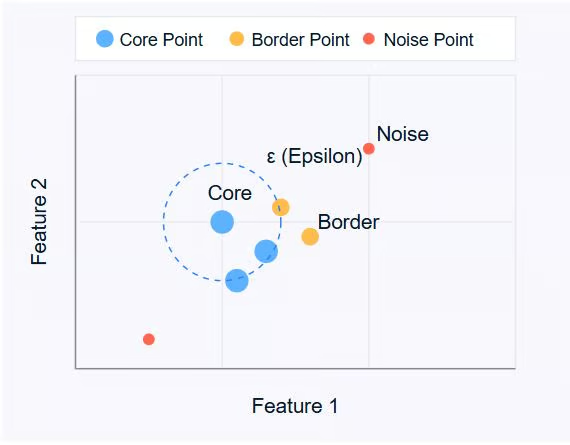
Image by author

The diagram above illustrates these concepts. Core points (blue) form the heart of clusters, border points (orange) are on the edge of clusters, and noise points (red) are isolated.

DBSCAN uses two main parameters:

• ε (epsilon): The maximum distance between two points for them to be considered as neighbors.
• MinPts: The minimum number of points required to form a dense region.

By adjusting these parameters, you can control how the algorithm defines clusters, allowing it to adapt to different types of datasets and clustering requirements.

In the next section, we'll look at how the DBSCAN algorithm works, exploring its step-by-step process for identifying clusters in data.

How Does DBSCAN Work?

DBSCAN operates by examining the neighborhood of each point in the dataset. The algorithm follows a step-by-step process to identify clusters based on the density of data points. Let's break down how DBSCAN works:

1. Parameter Selection
• Choose ε (epsilon): The maximum distance between two points for them to be considered as neighbors.
• Choose MinPts: The minimum number of points required to form a dense region.
2. Select a Starting Point
• The algorithm starts with an arbitrary unvisited point in the dataset.
3. Examine the Neighborhood
• It retrieves all points within the ε distance of the starting point.
• If the number of neighboring points is less than MinPts, the point is labeled as noise (for now).
• If there are at least MinPts points within ε distance, the point is marked as a core point, and a new cluster is formed.
4. Expand the Cluster
• All the neighbors of the core point are added to the cluster.
• For each of these neighbors:
• If it's a core point, its neighbors are added to the cluster recursively.
• If it's not a core point, it's marked as a border point, and the expansion stops.
5. Repeat the Process
• The algorithm moves to the next unvisited point in the dataset.
• Steps 3-4 are repeated until all points have been visited.
6. Finalize Clusters
• After all points have been processed, the algorithm identifies all clusters.
• Points initially labeled as noise might now be border points if they're within ε distance of a core point.
7. Handling Noise
• Any points not belonging to any cluster remain classified as noise.

This process allows DBSCAN to form clusters of arbitrary shapes and identify outliers effectively. The algorithm's ability to find clusters without specifying the number of clusters beforehand is one of its key strengths.

It's important to note that the choice of ε and MinPts can significantly affect the clustering results. In the next section, we'll discuss how to choose these parameters effectively and introduce methods like the k-distance graph for parameter selection.

DBSCAN Key Concepts and Parameters

To fully grasp how DBSCAN forms clusters, it's important to understand two key concepts: density reachability and density connectivity.

Density reachability

A point q is density-reachable from a point p if:

1. p is a core point (has at least MinPts within ε distance)

2. There is a chain of points p = p₁, ..., p_n = q where each p_i+1 is directly density-reachable from p_i.

In simpler terms, you can reach q from p by stepping through core points, where each step is no larger than ε.

Density connectivity

Two points p and q are density-connected if there exists a point o such that both p and q are density-reachable from o.

Density connectivity is the basis for forming clusters in DBSCAN. All points in a cluster are mutually density-connected, and if a point is density-connected to any point in the cluster, it also belongs to that cluster.

Choosing DBSCAN Parameters

The effectiveness of DBSCAN heavily depends on the choice of its two main parameters: ε (epsilon) and MinPts. Here's how to approach selecting these parameters:

Selecting ε (Epsilon)

The ε parameter determines the maximum distance between two points for them to be considered neighbors. To choose an appropriate ε:

1. Use domain knowledge: If you have insight into what distance is meaningful for your specific problem, use that as a starting point.

2. K-distance graph: This is a more systematic approach:

• Calculate the distance to the k-th nearest neighbor for each point (where k = MinPts).
• Plot these k-distances in ascending order.
• Look for an "elbow" in the graph – a point where the curve starts to level off.
• The ε value at this elbow is often a good choice.

Selecting MinPts

MinPts determines the minimum number of points required to form a dense region. Here are some guidelines:

1. General rule: A good starting point is to set MinPts = 2 * num_features, where num_features is the number of dimensions in your dataset.

2. Noise consideration: If your data has noise or you want to detect smaller clusters, you might want to decrease MinPts.

3. Dataset size: For larger datasets, you might need to increase MinPts to avoid creating too many small clusters.

Remember, the choice of parameters can significantly affect the results. It's often beneficial to experiment with different values and evaluate the resulting clusters to find the best fit for your specific dataset and problem.

Implementing DBSCAN in Python

In this section, we'll look at the implementation of DBSCAN using Python and the scikit-learn library. We'll use the Make Moons dataset to demonstrate the process.

Setting up the environment

import numpy as np
import matplotlib.pyplot as plt
from sklearn.datasets import make_moons
from sklearn.cluster import DBSCAN
from sklearn.neighbors import NearestNeighbors

These imports provide the necessary tools for data manipulation, visualization, dataset creation, and implementing the DBSCAN algorithm.

Generating sample data

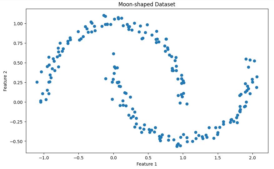
X, _ = make_moons(n_samples=200, noise=0.05, random_state=42)

This code creates a synthetic dataset using the make_moons function from scikit-learn. Here's a brief description of the dataset:

The make_moons function generates a binary classification dataset that resembles two interleaving half moons. In our case:

• We create 200 samples (n_samples=200)
• We add a small amount of Gaussian noise (noise=0.05) to make the dataset more realistic
• We set random_state=42 for reproducibility

This dataset is particularly useful for demonstrating DBSCAN because:

1. It has a non-convex shape that many clustering algorithms (like K-means) would struggle with
2. The two clusters are clearly separated but have a complex shape
3. The added noise provides a more realistic scenario where some points might be classified as outliers

Let's visualize this dataset to better understand its structure:

# Visualize the dataset
plt.figure(figsize=(10, 6))
plt.scatter(X[:, 0], X[:, 1])
plt.title('Moon-shaped Dataset')
plt.xlabel('Feature 1')
plt.ylabel('Feature 2')
plt.show()

This will show you the two interleaving half-moon shapes in our dataset as shown below

Determining the epsilon parameter

We use the k-distance graph method to help choose an appropriate epsilon value:

1. We define a function plot_k_distance_graph that calculates the distance to the k-th nearest neighbor for each point.
2. The distances are sorted and plotted.
3. We look for an "elbow" in the resulting graph to choose epsilon.

# Function to plot k-distance graph
def plot_k_distance_graph(X, k):
    neigh = NearestNeighbors(n_neighbors=k)
    neigh.fit(X)
    distances, _ = neigh.kneighbors(X)
    distances = np.sort(distances[:, k-1])
    plt.figure(figsize=(10, 6))
    plt.plot(distances)
    plt.xlabel('Points')
    plt.ylabel(f'{k}-th nearest neighbor distance')
    plt.title('K-distance Graph')
    plt.show()
# Plot k-distance graph
plot_k_distance_graph(X, k=5)

Output

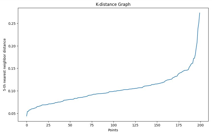
In our example, based on the k-distance graph, we choose an epsilon of 0.15.

Performing DBSCAN clustering

We use scikit-learn's DBSCAN implementation:

1. We set epsilon=0.15 based on our k-distance graph.
2. We set min_samples=5 (2 * num_features, as our data is 2D).
3. We fit the model to our data and predict the clusters.

# Perform DBSCAN clustering
epsilon = 0.15  # Chosen based on k-distance graph
min_samples = 5  # 2 * num_features (2D data)
dbscan = DBSCAN(eps=epsilon, min_samples=min_samples)
clusters = dbscan.fit_predict(X)

Visualizing the results

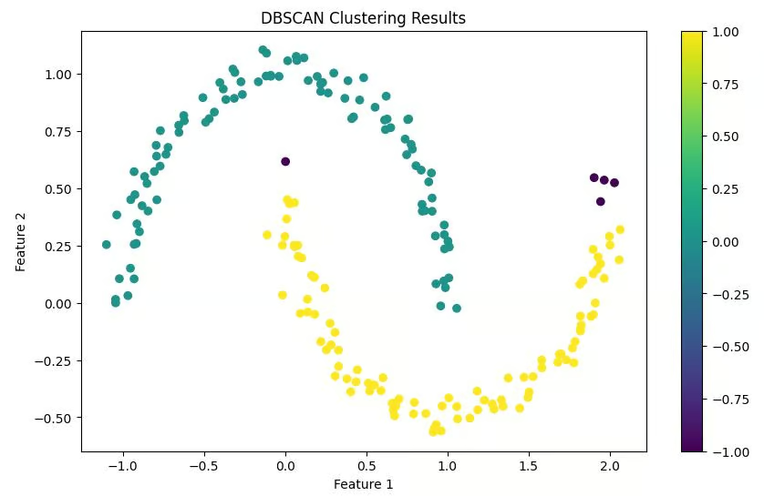
We create a scatter plot of our data points, coloring them according to their assigned clusters. Points classified as noise are typically colored differently (often black).

# Visualize the results
plt.figure(figsize=(10, 6))
scatter = plt.scatter(X[:, 0], X[:, 1], c=clusters, cmap='viridis')
plt.colorbar(scatter)
plt.title('DBSCAN Clustering Results')
plt.xlabel('Feature 1')
plt.ylabel('Feature 2')
plt.show()

Output

Interpreting the results

Finally, we print out the number of clusters found and the number of points classified as noise. This gives us a quick summary of the clustering results.

# Print number of clusters and noise points
n_clusters = len(set(clusters)) - (1 if -1 in clusters else 0)
n_noise = list(clusters).count(-1)
print(f'Number of clusters: {n_clusters}')
print(f'Number of noise points: {n_noise}')

Output

Number of clusters: 2

Number of noise points: 5

This implementation provides a complete workflow from data generation to results interpretation. It's important to note that in real-world scenarios, you would replace the sample data generation with loading and preprocessing your actual dataset.

Remember, the key to successful DBSCAN clustering often lies in appropriate parameter selection. Don't hesitate to experiment with different epsilon and min_samples values to find the best fit for your specific dataset.

DBSCAN vs. K-Means

While both DBSCAN and K-Means are popular clustering algorithms, they have distinct characteristics that make them suitable for different types of data and use cases. Let's compare these two algorithms to understand when to use each one.

Visual comparison

To illustrate these differences, let's apply both algorithms to our moon-shaped dataset

from sklearn.cluster import KMeans

# DBSCAN clustering
dbscan = DBSCAN(eps=0.15, min_samples=5)
dbscan_labels = dbscan.fit_predict(X)

# K-Means clustering
kmeans = KMeans(n_clusters=2, random_state=42)
kmeans_labels = kmeans.fit_predict(X)

# Visualize the results
fig, (ax1, ax2) = plt.subplots(1, 2, figsize=(15, 6))

ax1.scatter(X[:, 0], X[:, 1], c=dbscan_labels, cmap='viridis')
ax1.set_title('DBSCAN Clustering')

ax2.scatter(X[:, 0], X[:, 1], c=kmeans_labels, cmap='viridis')
ax2.set_title('K-Means Clustering')

plt.show()

This code applies both DBSCAN and K-Means to our dataset and visualizes the results side by side.

Output

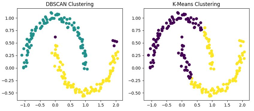
You'll notice that

1. DBSCAN correctly identifies the two half-moon shapes as separate clusters.
2. K-Means struggles with the non-convex shape, often splitting one moon into two clusters or combining parts of both moons into one cluster.
3. DBSCAN may identify some points as noise (usually colored differently), while K-Means assigns every point to a cluster.

When to use DBSCAN?

Now that we've seen how DBSCAN works and compared it to K-Means, let’s see when DBSCAN is the right choice for our clustering needs. The unique properties of DBSCAN make it particularly well-suited for certain types of data and problem domains.

Complex cluster shapes 

Building on our previous comparison, DBSCAN truly shines when dealing with non-globular cluster shapes. If your data forms arbitrary patterns like the half-moons we explored earlier, DBSCAN is likely to outperform traditional algorithms like K-Means. 

For example, in geographical analysis, natural formations like river systems or urban sprawl often form irregular shapes that DBSCAN can effectively identify.

Unknown number of clusters

One of DBSCAN's key advantages is its ability to determine the number of clusters automatically. This is particularly useful in exploratory data analysis where you might not have prior knowledge about the underlying structure of your data. 

Consider a market segmentation problem: you might not know in advance how many distinct customer groups exist. DBSCAN can help uncover these segments without requiring you to guess the number of clusters.

Datasets with noise 

DBSCAN's approach to handling noise points makes it robust to outliers. This is crucial in many real-world datasets where measurement errors or anomalies are common.

For instance, in anomaly detection systems for network security, DBSCAN can effectively separate normal network traffic patterns from potential security threats.

Varying cluster densities

Unlike K-Means, which assume clusters of similar density, DBSCAN can identify clusters of varying densities. This is particularly useful in scenarios where some groups in your data are more tightly packed than others.

An example could be analyzing galaxy distributions in astronomy, where different regions of space have varying densities of celestial objects.

While DBSCAN is powerful, it's important to be aware of its limitations:

1. Parameter Sensitivity: As we discussed earlier, choosing appropriate values for ε and MinPts is crucial. Poor choices can lead to suboptimal clustering results.
2. High-Dimensional Data: DBSCAN's performance can degrade with high-dimensional data due to the "curse of dimensionality."
3. Varying Densities: While DBSCAN can handle clusters of different densities, extremely varying densities in the same dataset can still pose challenges.
4. Scalability: For very large datasets, DBSCAN might be computationally expensive compared to algorithms like K-Means.

In the next section, we’ll look at some practical applications of DBSCAN.

Practical Examples of DBSCAN

DBSCAN finds applications across various domains.

Spatial data analysis

In geographic information systems (GIS), DBSCAN can identify areas of high activity or interest. For instance, a study titled ‘Uncovering urban human mobility from large scale taxi GPS data’ demonstrates how DBSCAN can detect urban hotspots from taxi GPS data. 

This application showcases DBSCAN's ability to identify dense activity regions in spatial data, which is crucial for urban planning and transportation management.

Image processing 

DBSCAN can group pixels into distinct objects for tasks like object recognition in images. A study titled 'Segmentation of Brain Tumour from MRI Image – Analysis of K-means and DBSCAN Clustering' demonstrates DBSCAN's effectiveness in medical image analysis. 

The researchers used DBSCAN to accurately segment brain tumors in MRI scans, showcasing its potential in computer-aided diagnosis and medical imaging.

Anomaly detection 

In fraud detection or system health monitoring, DBSCAN can isolate unusual patterns. A study titled 'Efficient density and cluster-based incremental outlier detection in data streams' demonstrates the application of a modified DBSCAN algorithm for real-time anomaly detection. 

The researchers applied an incremental version of DBSCAN to detect outliers in streaming data, which has potential applications in fraud detection and system health monitoring. 

This study showcases how DBSCAN can be adapted for identifying unusual patterns in continuous data streams, a crucial capability for real-time fraud detection systems.

Recommendation systems

DBSCAN can group users with similar preferences, helping to generate more accurate recommendations. For example, a study titled "Multi-Cloud Based Service Recommendation System Using DBSCAN Algorithm" demonstrates the application of DBSCAN in improving collaborative filtering for recommendation systems. The researchers used DBSCAN as part of a clustering approach to group users based on their movie preferences and ratings, which improved the accuracy of movie recommendations.

This approach showcases how DBSCAN can enhance personalized recommendations in domains such as entertainment streaming services.

Conclusion

DBSCAN is a powerful tool in the data scientist's toolkit, particularly valuable when dealing with complex, noisy datasets where the number of clusters is unknown. However, like any algorithm, it's not a one-size-fits-all solution. 

The key to successful clustering lies in understanding your data, the strengths and limitations of different algorithms, and choosing the right tool for the job. In many cases, trying multiple clustering approaches, including DBSCAN and K-Means, and comparing their results can provide valuable insights into your data's structure.

With practice and experience, you'll develop an intuition for when DBSCAN is likely to unveil the hidden patterns in your data.

You can learn more about the various technologies and methods we’ve covered in this post on DataCamp with the following resources: 

• Machine Learning Scientist in Python
• Unsupervised Machine Learning Cheat Sheet
• Unsupervised Learning in Python Course