Understanding the Exponential Distribution: A Comprehensive Guide

Understanding probability distributions is fundamental to data science, and among these, I find the exponential distribution stands out as one with some unique features worth exploring. While it shares mathematical connections with the Poisson distribution, the exponential distribution uniquely models time intervals between events rather than event counts. 

For those new to probability concepts, our Foundations of Probability in Python course provides essential background knowledge. The exponential distribution's practical applications extend across various domains, from reliability engineering to queueing theory, making it particularly valuable in fields like survival analysis, which is explored in depth in Survival Analysis in Python. This guide will explore the fundamental concepts, mathematical foundations, and real-world applications of the exponential distribution, equipping you with the knowledge to effectively apply it in your data science projects.

What is the Exponential Distribution?

The exponential distribution is a continuous probability distribution that models the time between events in a process where events occur continuously and independently at a constant average rate. It's particularly useful for analyzing situations involving waiting times, lifetimes, and intervals between events.

Imagine you're working at a busy customer service center. The time between incoming customer calls often follows an exponential distribution. Similarly, in manufacturing, the time until a machine fails or needs maintenance frequently exhibits exponential behavior.

Key characteristics of the exponential distribution

The exponential distribution has several unique properties that make it particularly useful in real-world applications:

The memoryless property

This is perhaps the most distinctive characteristic of the exponential distribution. It means that the future behavior of the system doesn't depend on its past history. For example, if a light bulb has already lasted for 1000 hours, the probability it will last another 100 hours is the same as if it were brand new. This property is unique to the exponential distribution among continuous distributions.

Constant hazard rate

The exponential distribution maintains a constant failure rate over time. This means the probability of an event occurring in the next small time interval remains the same, regardless of how much time has passed.

The relationship between the exponential and Poisson distributions is fundamental in probability theory. While the Poisson distribution models the number of events occurring in a fixed time interval, the exponential distribution models the time between these events. They're two sides of the same coin: if events occur according to a Poisson process with rate λ, then the waiting time between events follows an exponential distribution with parameter λ.

Mathematical formulation

The exponential distribution is defined by a single parameter λ (lambda), which represents the rate parameter. Let's look at its key mathematical components:

Probability density function (PDF)

The PDF helps us calculate the probability of an event occurring within a specific interval. The PDF for the exponential distribution is as follows:   

   where:

• x is the random variable (typically representing time)
• λ is the rate parameter (λ > 0)
• e is Euler's number (approximately 2.71828)

Cumulative Distribution Function (CDF)

The CDF is particularly useful when we want to find the probability of an event occurring before a certain time. It gives us the probability that the waiting time is less than or equal to a specific value. Here is the CDF for the exponential distribution:

Applications of the Exponential Distribution

The exponential distribution plays a vital role in various fields, helping us model and understand time-dependent processes. Let's explore some of its key applications. 

Reliability engineering

Reliability engineering relies heavily on the exponential distribution to model the lifespan of components and systems. This is particularly useful because of the distribution's "memoryless" property - the future lifetime of a component depends only on the present, not how long it has already been operating.

For example, electronic components typically exhibit exponentially distributed failure times, demonstrating the unique memoryless property of this distribution. This means a new microprocessor has the same probability of failing in the next hour as one that has been running for a month (assuming no wear-out effects). Server hardware manufacturers extensively use this distribution in their reliability analyses to calculate Mean Time Between Failures (MTBF), determine optimal maintenance schedules, and predict warranty costs and replacement needs. This information is valuable for both product development and business planning.

Queueing theory

In queueing theory, the exponential distribution is fundamental for modeling the time between arrivals or service times in many systems. This application is particularly useful in:

1. Customer Service Centers:

• Modeling time between incoming calls
• Predicting peak load times
• Optimizing staff scheduling

2. Telecommunications:

• Analyzing network traffic patterns
• Modeling packet arrival times in data networks
• Planning network capacity

3. Healthcare Systems:

• Modeling patient arrival times in emergency departments
• Estimating wait times for services
• Planning resource allocation

The exponential distribution works well in these contexts because many arrival processes can be approximated as memory-less events occurring at a constant average rate.

Calculating Probabilities with the Exponential Distribution

When working with the exponential distribution, we have two main approaches for calculating probabilities: the PDF is particularly useful when we need to find the probability of an event occurring within a specific interval or range, while the CDF helps us determine the probability of an event occurring before a certain point in time. Let's explore both approaches using a practical help desk scenario.

Using the probability density function

We mentioned that the PDF helps us calculate the probability of an event occurring within an interval. For continuous distributions like the exponential, we need to integrate the PDF over the interval of interest.

Let's work through a practical example: Imagine we're analyzing customer service calls at a help desk where calls arrive following an exponential distribution with an average rate of 3 calls per hour (λ = 3).

To find the probability of waiting between 10 and 20 minutes for the next call, we would:

1. Convert time to hours: (10 minutes = 1/6 hour, 20 minutes = 1/3 hour)
2. Use the formula: P(1/6 < X < 1/3) = ∫[1/6 to 1/3] 3e^(-3x)dx
3. Evaluate: = -e^{(-3x)|[1/6 to 1/3]}
4. Calculate: = [e^(-0.5) - e^(-1)] ≈ 0.2325 or about 23.25%

Using the cumulative distribution function

We said that the CDF is useful when we want to find the probability of an event before a time. Now, using our help desk example: What's the probability that we'll receive a call within the first 15 minutes?

Using our help desk example: What's the probability that we'll receive a call within the first 15 minutes?

1. Convert 15 minutes to hours: (15 minutes = 1/4 hour)
2. Use the CDF formula: F(1/4) = 1 - e^(-3*1/4)
3. Calculate: = 1 - e^(-0.75) ≈ 0.5276 or about 52.76%

This means there's roughly a 53% chance of receiving a call within the first 15 minutes. Notice how the CDF makes these "up to" probability calculations more straightforward than using the PDF.

Visualizing the Exponential Distribution

Let's first look at the exponential distribution by itself and then compare it to other distributions.

Graphical representation

Here is a set of graphs I created in Python:

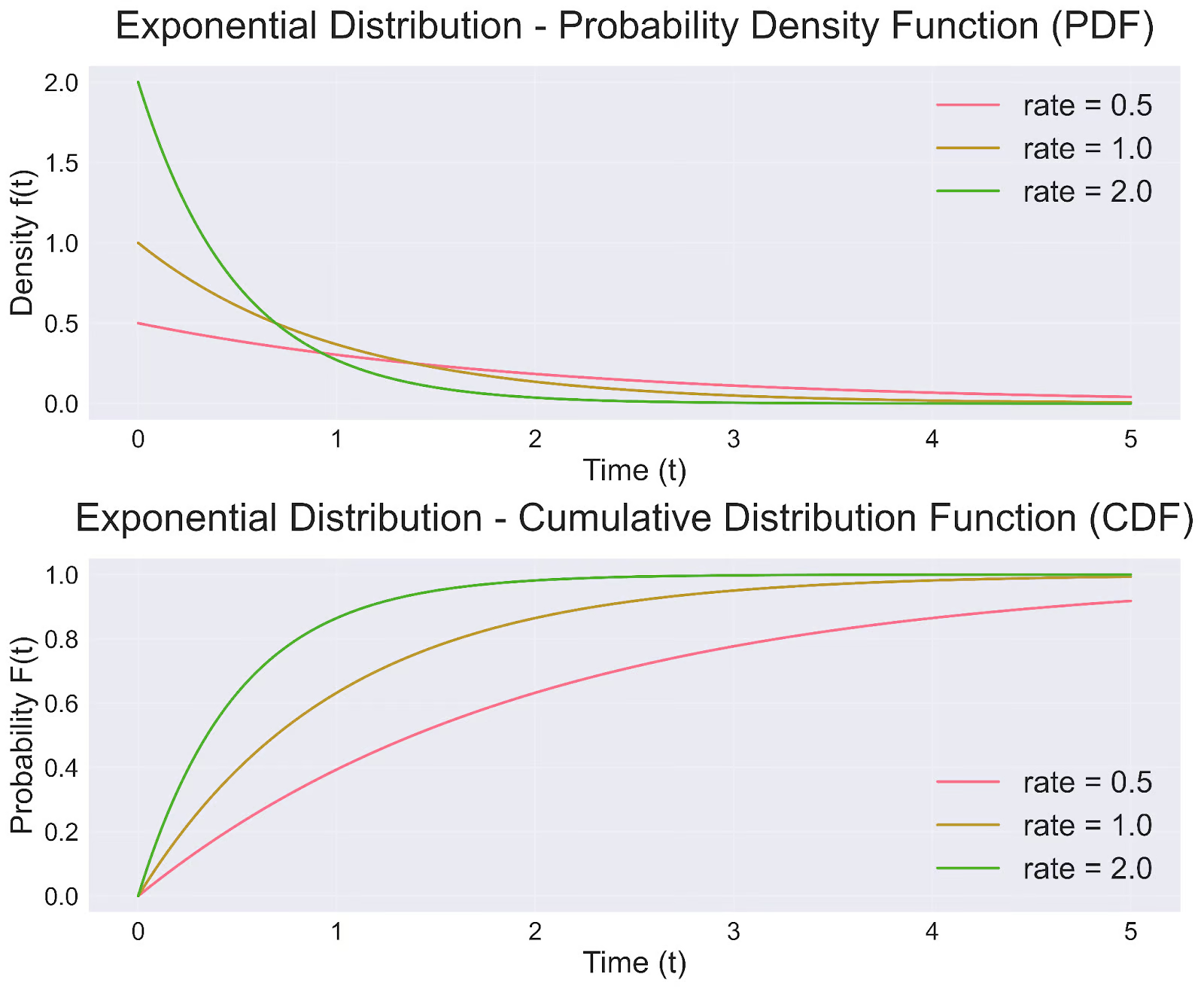
Let's explore how the mathematical formulas translate into visual patterns. The visualization shows three different rate parameters (0.5, 1.0, and 2.0) to demonstrate how λ shapes the distribution:

Looking at the PDF (top graph):

• When λ = 2.0 (green line), we see the steepest initial decline, starting at f(0) = 2.0. This indicates that early events are much more likely
• When λ = 1.0 (orange line), we get the standard exponential distribution with a more moderate decay
• When λ = 0.5 (red line), the curve declines more gradually, showing that longer waiting times are more common

The CDF (bottom graph) tells a complementary story:

• The higher rate (λ = 2.0) results in the steepest rise, showing that cumulative probability accumulates quickly
• The lower rate (λ = 0.5) shows a more gradual accumulation of probability
• All curves eventually approach 1, illustrating that the probability of the event occurring approaches certainty as time increases

This behavior makes the exponential distribution particularly useful for modeling real-world phenomena like waiting times, equipment lifetimes, and time between events in a Poisson process.

Comparing with other distributions

The exponential distribution's unique characteristics become clearer when compared with other common probability distributions. Let's examine these comparisons through our visualization:

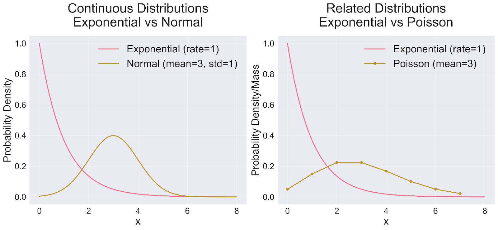
When examining the normal distribution comparison (left panel), several key differences emerge. The exponential distribution exhibits a pronounced right skew, reaching its peak value immediately before declining continuously. This contrasts sharply with the normal distribution's familiar symmetric, bell-shaped curve centered around its mean value. Though both qualify as continuous distributions, they serve distinct modeling purposes: the exponential distribution excels at modeling waiting times and intervals, while the normal distribution typically handles measurements and averages.

The relationship with the Poisson distribution (right panel) reveals another fascinating dimension of probability theory. Where the exponential distribution measures the time between events, the Poisson distribution focuses on counting the number of events within a fixed interval. These distributions form two sides of the same coin: in a Poisson process, the waiting times naturally follow an exponential distribution. Another notable distinction lies in their continuity - the exponential distribution can take any positive real value, while the Poisson distribution deals exclusively with discrete, non-negative integers.

These comparative insights illuminate why the exponential distribution excels in specific modeling scenarios. It proves invaluable when analyzing time intervals between random events, offering capabilities beyond the Poisson distribution's event-counting focus. The distribution particularly shines in scenarios demanding immediate occurrence probability assessment, contrasting with the normal distribution's central tendency approach. Perhaps most distinctively, its unique memoryless property sets it apart from both Normal and Poisson distributions, making it the optimal choice for processes where past events don't influence future probabilities.

Common Misconceptions and Pitfalls

When working with the exponential distribution, several common misconceptions can lead to incorrect analysis. Understanding these potential pitfalls helps ensure accurate application of the distribution in real-world scenarios.

Misinterpreting the memoryless property

The memoryless property often causes confusion because it seems to contradict our everyday experience. Here are common misunderstandings and their corrections:

One frequent misconception is thinking that the memoryless property means past events have no value for prediction. In reality, it means that the probability of waiting an additional time period remains the same, regardless of how long you've already waited. For example:

• Incorrect interpretation: "If a light bulb follows an exponential distribution and hasn't failed in 5 years, it must be about to fail soon."
• Correct interpretation: "If a light bulb follows an exponential distribution and hasn't failed in 5 years, its probability of lasting another year is the same as a new bulb lasting a year."

Another misconception involves assuming all reliability scenarios exhibit the memoryless property. In reality, many systems show aging effects or wear-out patterns that don't follow exponential behavior. For instance, mechanical components often have increasing failure rates over time.

Incorrect parameter usage

Several common mistakes occur when selecting and applying the rate parameter:

1. Rate vs. mean confusion:

   • A common error is using the mean value as the rate parameter (λ)

   • Remember: The mean (expected value) is actually 1/λ

   • For example, if events occur on average every 2 hours, λ = 1/2, not 2

2. Unit mismatch:

   • The rate parameter must be consistent with the time units in your data

   • If you measure time in hours but specify λ in days^(-1), your probabilities will be incorrect

   • Always convert to consistent units before applying the distribution

3. Over-application:

   • Verfity that events occur independently

   • That the rate remains constant over time

   • And that the process has no memory effects 

To avoid these errors, always clearly define your units and convert them consistently, verify that the assumptions of exponential distribution fit your scenario, test your data for exponential behavior before applying the distribution, and document your parameter choices and their justification.

Conclusion

The exponential distribution's elegant simplicity and powerful applications make it an indispensable tool in a data scientist's toolkit. Its unique memoryless property and relationship with other distributions, particularly the Gaussian distribution, highlight its special place in probability theory.

While this guide has covered the essential aspects, there's always more to explore in specialized applications. For those interested in practical implementations, our Statistical Simulation in Python course offers hands-on experience with these concepts. Additionally, understanding how the exponential distribution relates to other probability distributions, as detailed in Multivariate Probability Distributions in R, provides a broader perspective on its role in statistical modeling. Whether you're analyzing survival data, modeling system reliability, or studying queue behaviors, mastering the exponential distribution opens up new possibilities in data analysis and statistical modeling.