Feature Extraction in Machine Learning: A Complete Guide

Feature extraction in machine learning transforms raw data into a set of meaningful characteristics, capturing essential information while reducing redundancy. It can involve dimensionality reduction techniques and methods that create new features from existing data.

Imagine you're trying to identify fruits in a market. While you could consider countless attributes (weight, color, texture, shape, smell, etc.), you might realize that just a few key features like color and size are enough to distinguish between apples and oranges. This is exactly what feature extraction does. It helps you focus on the most informative characteristics of your data.

When performing feature extraction, the original data is mathematically transformed into a new set of features. These new features are designed to capture the most important aspects of the data while potentially reducing its complexity. The extracted features often represent underlying patterns or structures that might not be immediately apparent in the original data.

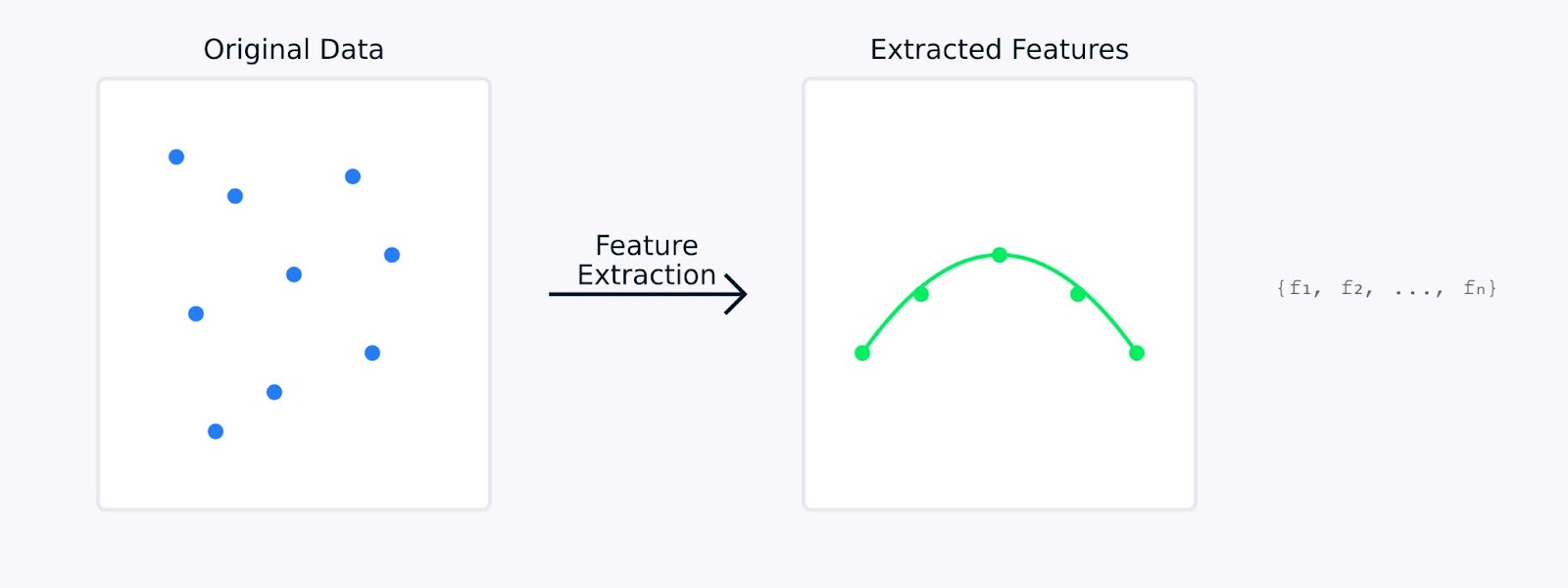
Feature Extraction

In the next sections, we'll explore why feature extraction is so important in machine learning and look into various methods for extracting features from different types of data along with their code. If you want some hands-on examples, check out our Dimensionality Reduction in Python course, which has a chapter dedicated to feature extraction.

Why is Feature Extraction important in Machine Learning?

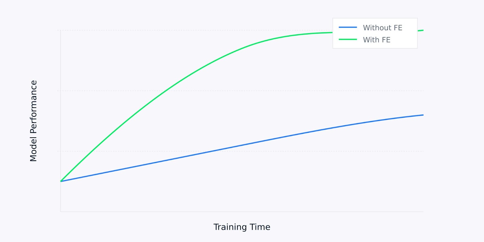
Feature extraction plays an important role in machine learning. It can make the difference between a model that fails and one that succeeds. Let's see why this is so fundamental to building effective machine learning models.

Enhancing model accuracy and efficiency

When working with raw data, machine learning models often struggle to distinguish between meaningful patterns and noise. Feature extraction serves as a data preprocessing step that can significantly improve how well your models learn and perform.

Model Performance versus Training Time

For example, when a model achieves 85% accuracy with raw data, the same model might reach 95% accuracy when trained on carefully extracted features. This improvement comes not from changing the model but from giving it better-quality input data from which to learn.

Managing high-dimensional datasets

Modern datasets often come with hundreds or thousands of features. This brings several challenges that feature extraction helps address.

• The curse of dimensionality: As the number of features increases, the data becomes increasingly sparse in the feature space. This makes it harder for models to find meaningful patterns. Feature extraction creates a more compact representation that preserves important relationships while reducing the dimensionality.
• High memory usage: High-dimensional data requires more storage and memory during processing. By extracting only the most relevant features, we can significantly reduce the memory footprint of our datasets while maintaining their informative value.
• Data visualization: It's impossible to visualize data with more than three dimensions directly. Feature extraction can reduce the dimensionality to two or three features, making it possible to plot and understand the data structure visually.

Feature extraction addresses these challenges by reducing the dimensionality while preserving essential information. This reduction transforms sprawling, high-dimensional data into a more compact and manageable form, leading to increased model performance.

Reducing computational complexity and preventing overfitting

Feature extraction provides two critical benefits for machine learning models:

1. Lower computational requirements
1. Fewer features mean faster training times
2. Reduced memory usage during model deployment
3. More efficient prediction generation
2. Better generalization
1. Simpler feature spaces help prevent overfitting
2. Models learn more robust patterns
3. Improved performance on new, unseen data

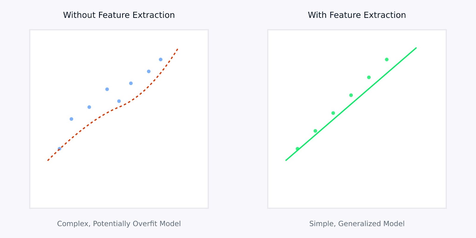
Feature Extractions versus Without Feature Extraction

The visualization above illustrates how feature extraction can lead to simpler, more robust models. The left plot shows a complex model trying to fit noisy, high-dimensional data, while the right plot shows how feature extraction can reveal a clearer, more generalizable pattern.

Working with extracted features rather than raw data is like giving your model a clear, distilled version of the information it needs to learn from. This not only makes the learning process more efficient but also leads to models that are more likely to perform well in real-world applications.

Next, let’s see different methods of feature extraction.

Methods of Feature Extraction

Feature extraction methods can be broadly categorized into two main approaches: manual feature engineering and automated feature extraction. Let's look at both these methods to understand how they help transform raw data into meaningful features.

Manual feature engineering

Manual feature engineering involves using domain expertise to identify and create relevant features from raw data. This hands-on approach relies on our understanding of the problem and the data to craft meaningful features.

In image processing, manual feature engineering might involve techniques such as edge detection to identify object boundaries, color histograms to capture color distribution, texture analysis to quantify patterns, and shape descriptors to characterize object geometry.

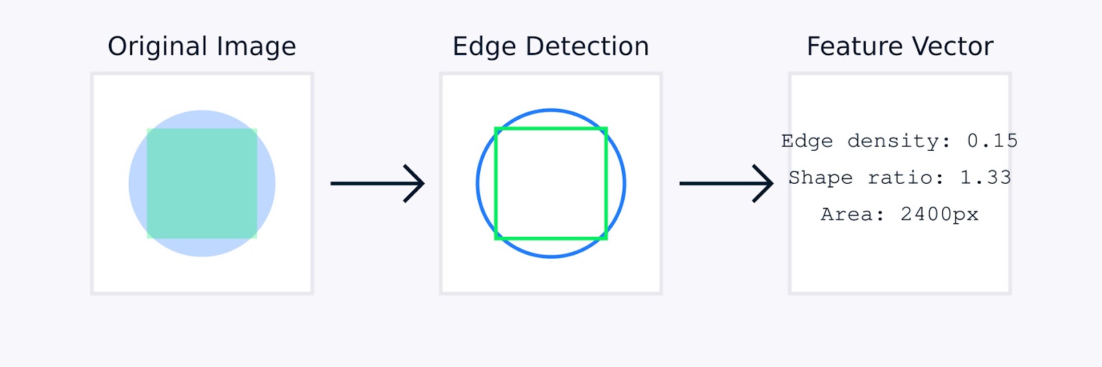
Image Feature Extraction

For tabular data, manual feature engineering involves creating interaction terms between existing features, transforming variables using logarithmic or polynomial functions, aggregating data points into meaningful statistics, and encoding categorical variables. 

Tabular data feature extraction

These techniques, guided by domain expertise, enhance the quality of the data representation and can significantly improve model performance.

Automated feature extraction

Automated feature extraction uses algorithms to discover and create features without explicit human guidance. These methods are particularly useful when dealing with complex datasets where manual feature engineering might be impractical or inefficient.

Common automated approaches include:

Principal Component Analysis (PCA): Transforms data into a set of uncorrelated components, with each component capturing the maximum remaining variance. This approach is particularly useful for dimensionality reduction, as it preserves the essential information within the data while simplifying its structure.

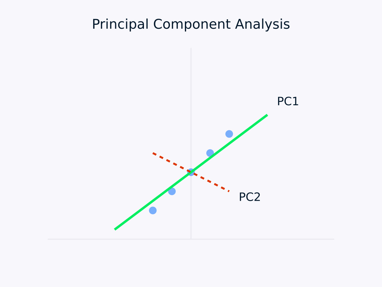
Principal Component Analysis (PCA)

Autoencoders: These are neural networks that learn compressed representations of data, capturing non-linear relationships. They are particularly effective for high-dimensional datasets, where traditional linear methods might fall short.

Various tools and libraries have emerged to simplify feature engineering tasks. For example, Scikit-learn's decomposition module offers a range of methods for dimensionality reduction, and PyCaret provides automated feature selection capabilities.

Both manual and automated approaches have their strengths. Let’s look at the strengths of each approach.

The choice between manual and automated methods often depends on factors such as dataset complexity, the availability of domain expertise, interpretability requirements, computational resources, and time constraints.

For highly complex datasets or when time and resources are limited, automated methods can quickly generate useful features. Conversely, manual methods may be preferable when domain expertise is available and interpretability is a priority, allowing for tailored feature engineering that aligns closely with the problem at hand.

In practice, many successful machine learning projects combine both approaches, using domain expertise to guide feature engineering while leveraging automated methods to discover additional patterns that might not be immediately apparent to human experts.

In the next section, we’ll look at several feature extraction techniques in various domains.

Feature Extraction Techniques

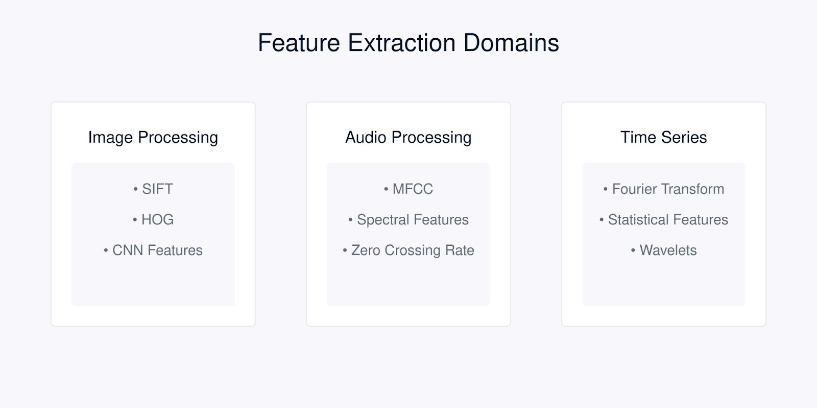
Each type of data requires specific feature extraction techniques optimized for its unique characteristics. Let's look at the most common techniques for different types of data.

Feature Extraction Techniques

Image feature extraction

Image feature extraction transforms raw pixel data into meaningful representations that capture essential visual information. There are three main categories of techniques used in modern computer vision. They are the traditional methods, deep learning based methods, and statistical methods.

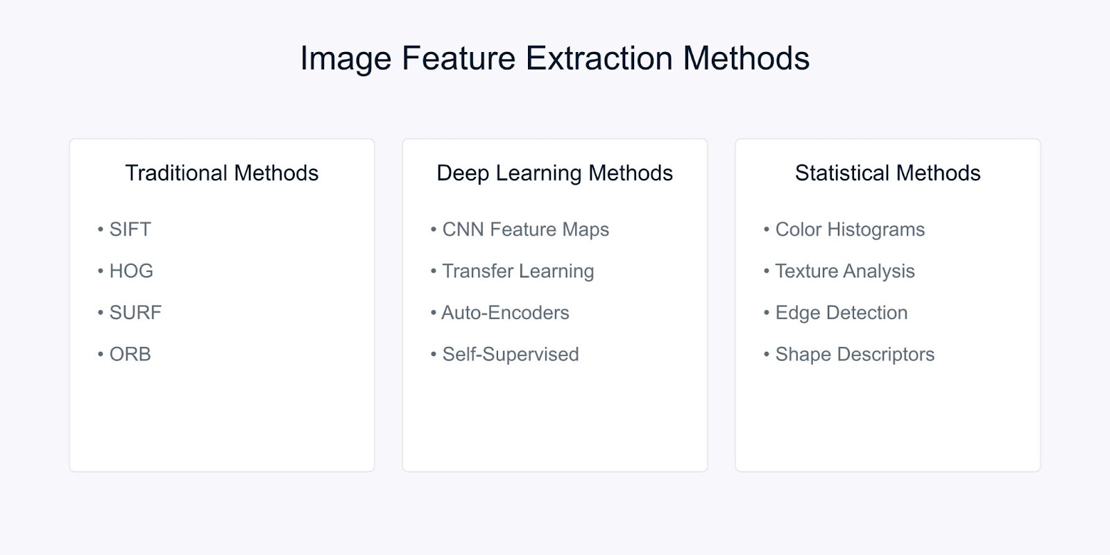
Image Feature Extraction Methods

Let’s look at each of the methods.

Traditional computer vision methods

Scale-Invariant Feature Transform (SIFT) is a robust method that detects distinctive local features in images. It works by identifying key points and generating descriptors that are:

• Invariant to image scaling and rotation
• Partially invariant to illumination changes
• Robust to local geometric distortion

The SIFT algorithm processes images through several stages. It begins with scale-space extrema detection to identify potential key points that are invariant to scale. Next, keypoint localization refines these candidates by pinpointing their precise locations and discarding unstable points.

Following this, orientation assignment determines a consistent orientation for each key point, ensuring rotation invariance. Finally, keypoint descriptor generation creates distinctive descriptors based on local image gradients, facilitating robust matching between images.

Another method is the Histogram of Oriented Gradients (HOG). It captures local shape information by analyzing gradient patterns across an image. The process begins by computing gradients throughout the image to highlight edge details. 

The image is then divided into small cells, and for each cell, a histogram of gradient orientations is created to summarize the local structure. Finally, these histograms are normalized across larger blocks to ensure robustness against variations in illumination and contrast, resulting in a robust feature descriptor for tasks like object detection and recognition.

Deep learning methods

Convolutional Neural Networks (CNNs) have changed how we do feature extraction by automatically learning hierarchical representations.

Feature Extraction with CNN

CNNs learn features through their hierarchical structure. In the early layers, they detect basic visual elements such as edges and colors. The middle layers then combine these elements to recognize patterns and shapes, while the deeper layers capture complex objects and enable scene understanding.

Transfer learning allows us to use these pre-learned features from models trained on large datasets, making them particularly valuable when working with limited data.

Statistical methods

Statistical methods extract both global and local patterns from images, facilitating robust image analysis and interpretation. 

For instance, color histograms represent the distribution of colors within an image and provide rotation and scale-invariant features, making them particularly useful for tasks such as image classification and retrieval.

Texture analysis captures repeated patterns and surface characteristics using techniques like Gray Level Co-occurrence Matrices (GLCM), which are effective for applications including material recognition and scene classification.

Additionally, edge detection identifies boundaries and significant intensity changes through methods such as Sobel, Canny, and Laplacian operators, playing a crucial role in object detection and shape analysis.

The choice of feature extraction method depends on several factors. It should align with the specific requirements of your task, consider available computational resources, and account for the need for interpretability. 

Additionally, the characteristics of your dataset—such as its size, noise levels, and complexity—play a crucial role, as do the required invariance properties like scale, rotation, and illumination.

Audio feature extraction

Imagine trying to teach a computer to understand speech the way humans do. This is where Mel-Frequency Cepstral Coefficients (MFCC) come in.

MFCCs are special audio features that break down sound in a way similar to how our ears process it. They're particularly effective because they focus on the frequencies that humans are most sensitive to. Think of them as translating sound into a format that both computers and human hearing would find meaningful.

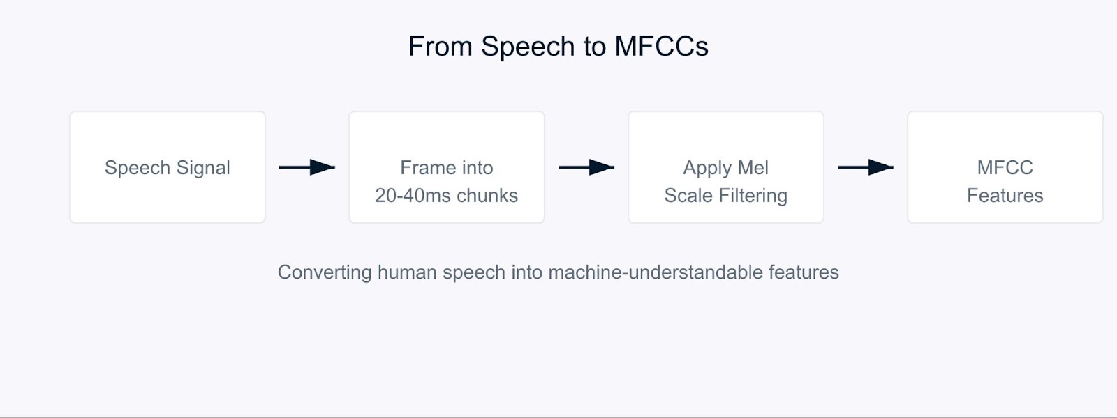
Mel-Frequency Cepstral Coefficients

The process starts by breaking down the audio signal into short chunks, typically 20-40 milliseconds long. For each chunk, we apply a series of mathematical transformations that convert the raw sound waves into frequency components. Here's where it gets interesting. Instead of treating all frequencies equally, we use something called the Mel scale.

This formula might look complex, but it's simply mapping frequencies to match how humans perceive sound. Our ears are better at detecting differences in lower frequencies than higher ones, and the Mel scale accounts for this natural bias.

In voice recognition, MFCCs serve as the foundation for understanding who's speaking and what they're saying. When you speak to your phone's virtual assistant, it's likely using MFCCs to process your voice. These coefficients help capture the unique characteristics of each person's voice, making them invaluable for speaker identification systems.

For sentiment analysis in speech, MFCCs help detect subtle variations in voice that indicate emotions. They can capture changes in pitch, tone, and speaking rate that might indicate whether someone is happy, sad, angry, or neutral. For example, when analyzing customer service calls, MFCCs can help identify customer satisfaction levels based on how they speak, not just what they say.

Time series feature extraction

When working with time series data, extracting meaningful features helps us capture patterns and trends that evolve over time. Let's look at some key techniques used to transform raw time series data into useful features.

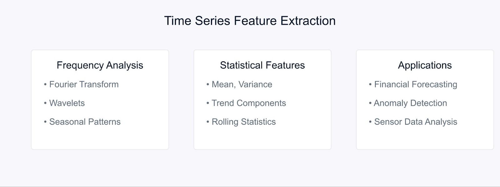
Time Series Feature Extraction Methods

The Fourier Transform decomposes time series data into its frequency components, revealing hidden periodic patterns. The formula is:

Statistical methods complement frequency analysis by capturing temporal characteristics. Common features include moving averages, standard deviations, and trend components. These techniques are particularly powerful in financial forecasting, where they help identify market trends and anomalies.

For example, in stock market analysis, combining Fourier features with statistical measures can reveal both long-term trends and cyclical patterns. Similarly, in industrial settings, these methods help detect equipment anomalies by analyzing sensor data patterns over time.

Tools and Libraries for Feature Extraction

Let’s look at some essential tools that make implementing these feature extraction methods straightforward and efficient.

Tools and Libraries for Feature Extraction

For image processing, OpenCV and scikit-image provide comprehensive tools for implementing various feature extraction techniques. These libraries offer efficient implementations of SIFT, HOG, and other algorithms we discussed earlier. When working with deep learning approaches, frameworks like TensorFlow and PyTorch become invaluable. You can get started with our OpenCV tutorial to learn more.

Audio processing tasks are simplified with libraries like LibROSA, which excels at extracting MFCCs and other acoustic features. PyAudioAnalysis extends these capabilities with high-level interfaces for audio analysis tasks.

For time series data, tsfresh and Featuretools automate the feature extraction process. These libraries can automatically generate and select relevant features from your temporal data, making it easier to focus on model development rather than feature engineering.

Example of Feature Extraction

Let's put our knowledge into practice with some hands-on examples. We'll start with image feature extraction, one of the most common applications in computer vision.

Image feature extraction using OpenCV 

First, let’s import the necessary libraries

# Import required libraries
import cv2
import numpy as np
import matplotlib.pyplot as plt

Now, let's load an image to extract relevant features. For this example, we'll use an image of Godzilla downloaded from the internet.

# Load the image
image = cv2.imread('godzilla.jpg')

# Convert BGR to RGB (OpenCV loads in BGR format)
image_rgb = cv2.cvtColor(image, cv2.COLOR_BGR2RGB)

# Display the original image
plt.imshow(image_rgb)
plt.title('Original Image')
plt.axis('off')
plt.show()

Output:

Before applying edge detection, we need to preprocess our image. We do that as follows:

# Convert the image to grayscale
gray_image = cv2.cvtColor(image, cv2.COLOR_BGR2GRAY)

# Apply Gaussian blur to reduce noise
blurred = cv2.GaussianBlur(gray_image, (5, 5), 0)

Finally, let's apply the Canny edge detection algorithm and visualize the results:

# Apply Canny edge detection
edges = cv2.Canny(blurred, threshold1=100, threshold2=200)

# Display the results
plt.figure(figsize=(10, 5))
plt.subplot(1, 2, 1)
plt.imshow(image_rgb)
plt.title('Original Image')
plt.axis('off')

plt.subplot(1, 2, 2)
plt.imshow(edges, cmap='gray')
plt.title('Edge Detection')
plt.axis('off')

plt.tight_layout()
plt.show()

Output:

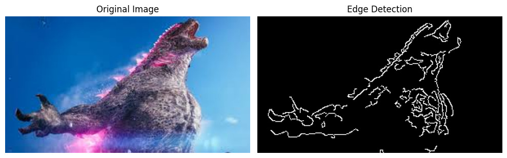
The Canny edge detector helps us identify important boundaries and features in our image, which can be used for further analysis or as input to machine learning models.

Extracting MFCC from audio using LibROSA

Before we can start processing audio files, we need to install the required libraries. Since LibROSA isn't included in Python's standard library, we'll use pip to install it:

# Install required libraries
# Run these commands in your terminal or command prompt
pip install librosa
pip install numpy
pip install matplotlib

LibROSA is a powerful library designed for music and audio analysis, so let's start by importing it along with other necessary libraries:

# Import required libraries
import librosa
import librosa.display
import numpy as np
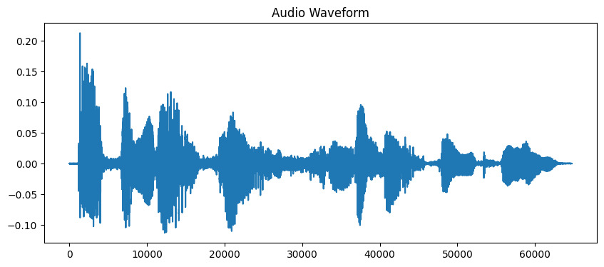
import matplotlib.pyplot as plt

Sound files contain a lot of information in waveform format. To work with this data, we first need to load it into our program. LibROSA helps us do this by converting the audio file into a format we can analyze:

# Load the audio file
# Duration is limited to 10 seconds for this example
audio_path = 'audio_sample.wav'
y, sr = librosa.load(audio_path, duration=10)

# Display the waveform
plt.figure(figsize=(10, 4))
plt.plot(y)
plt.title('Audio Waveform')
plt.show()

Output:

Now that we have our audio loaded, we need to extract meaningful features from it. Our ears naturally break down sound into different frequency components, and MFCC mimics this process. We use librosa's feature extraction function to compute these coefficients:

# Extract MFCC features
mfccs = librosa.feature.mfcc(y=y, sr=sr, n_mfcc=13)

# Display the MFCC
plt.figure(figsize=(10, 4))
librosa.display.specshow(mfccs, x_axis='time')
plt.colorbar(format='%+2.0f dB')
plt.title('MFCC')
plt.show()

Output:

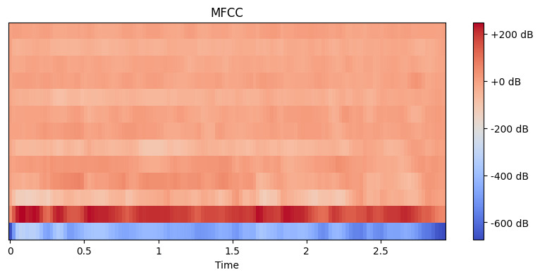
Here, we set n_mfcc=13 because the first 13 coefficients typically capture the most important aspects of sound that help in tasks like speech recognition. The resulting visualization shows how these features change over time, where brighter colors represent higher values.

Feature extraction from time series data with tsfresh

First, let's install the required libraries. We'll use the yfinance to get financial data, along with tsfresh for feature extraction:

# Install required libraries
# Run these commands in your terminal or command prompt
pip install tsfresh
pip install pandas
pip install numpy
pip install matplotlib
pip install yfinance

Now let's import our libraries and fetch some real financial data:

# Import required libraries
import pandas as pd
import numpy as np
from tsfresh import extract_features
from tsfresh.feature_extraction import MinimalFCParameters
import matplotlib.pyplot as plt
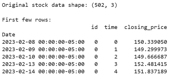
import yfinance as yf

Let's get some real stock market data. We'll use Apple's stock data as an example:

# Download Apple's stock data for the last 2 years
aapl = yf.Ticker("AAPL")
df = aapl.history(period="2y")

# Prepare the data in the format tsfresh expects
df_tsfresh = pd.DataFrame({
    'id': [0] * len(df),  # Each time series needs an ID
    'time': range(len(df)),
    'closing_price': df['Close']  # We'll use closing prices
})

# Display first few rows of our data
print("Original stock data shape:", df_tsfresh.shape)
print("\nFirst few rows:")
print(df_tsfresh.head())

Output:

Now let's extract features from our financial time series data:

# Set up the feature extraction parameters
extraction_settings = MinimalFCParameters()

# Extract features automatically
extracted_features = extract_features(df_tsfresh, 
                                   column_id='id', 
                                   column_sort='time',
                                   column_value='values',
                                   default_fc_parameters=extraction_settings)

# Display the extracted features
print("\nExtracted features shape:", extracted_features.shape)
print("\nExtracted features:")
print(extracted_features.head())

Output:

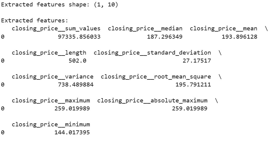
Here, we use MinimalFCParameters() to specify which features to extract. This gives us a basic set of meaningful time series features like mean, variance, and trend characteristics, which are essential for understanding patterns in our data.

Challenges in Feature Extraction

When working with feature extraction, we often encounter challenges.

High-dimensionality and computational constraints often arise when dealing with large datasets. For example, extracting features from high-resolution images or long audio files can consume significant memory and processing power.

Overfitting due to irrelevant or redundant features is another common challenge. When too many features are extracted, models might learn noise instead of meaningful patterns. This is especially common in image and audio processing where thousands of features can be generated.

To overcome these challenges, consider these strategies:

• Use domain knowledge to select relevant features
• Apply feature selection methods to reduce dimensionality
• Implement proper feature engineering techniques based on your data type

These challenges require careful consideration and balancing between feature richness and computational efficiency.

Conclusion

Feature extraction is a fundamental skill in machine learning that transforms raw data into meaningful representations. Through our practical examples with OpenCV, LibROSA, and tsfresh, we've seen how to extract features from different types of data. By understanding these techniques and their challenges, we can build effective machine learning models.

Ready to go deeper? Check out these resources:

• Feature Selection in Python Tutorial
• Feature Engineering for NLP in Python
• Dimensionality Reduction in Python
• Feature Engineering for Machine Learning in Python