
Course
Introduction to Data Engineering
4 hr
127.6K
Data preprocessing involves several steps, each addressing specific challenges related to data quality, structure, and relevance.
Let’s take a look at these key steps, which generally go in the following order:
Data cleaning is the process of identifying and correcting errors or inconsistencies in the data to ensure it is accurate and complete. The objective is to address issues that can distort analysis or model performance.
For example:
Here’s how it looks in Python:
# Creating a manual dataset
data = pd.DataFrame({
    'name': ['John', 'Jane', 'Jack', 'John', None],
    'age': [28, 34, None, 28, 22],
    'purchase_amount': [100.5, None, 85.3, 100.5, 50.0],
    'date_of_purchase': ['2023/12/01', '2023/12/02', '2023/12/01', '2023/12/01', '2023/12/03']
	})

# Handling missing values using mean imputation for 'age' and 'purchase_amount'
imputer = SimpleImputer(strategy='mean')
data[['age', 'purchase_amount']] = imputer.fit_transform(data[['age', 'purchase_amount']])

# Removing duplicate rows
data = data.drop_duplicates()

# Correcting inconsistent date formats
data['date_of_purchase'] = pd.to_datetime(data['date_of_purchase'], errors='coerce')

print(data)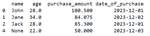
Output of code above
Data integration involves combining data from multiple sources to create a unified dataset. This is often necessary when data is collected from different source systems.
Some techniques used in data integration include:
For example, let’s say we have customer data from multiple databases. Here’s how we would merge it into a single view:
# Creating two manual datasets
data1 = pd.DataFrame({
    'customer_id': [1, 2, 3],
    'name': ['John', 'Jane', 'Jack'],
    'age': [28, 34, 29]
})

data2 = pd.DataFrame({
    'customer_id': [1, 3, 4],
    'purchase_amount': [100.5, 85.3, 45.0],
    'purchase_date': ['2023-12-01', '2023-12-02', '2023-12-03']
})

# Merging datasets on a common key 'customer_id'
merged_data = pd.merge(data1, data2, on='customer_id', how='inner')

print(merged_data)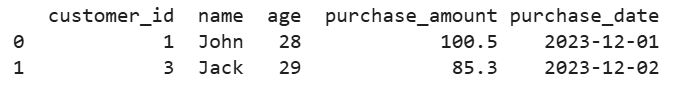
Output of code above
Data transformation converts data into formats suitable for analysis, machine learning, or mining.
For example:
Here’s how it looks in Python, using scikit-learn:
from sklearn.preprocessing import StandardScaler, OneHotEncoder

# Creating a manual dataset
data = pd.DataFrame({
    'category': ['A', 'B', 'A', 'C', 'B'],
    'numeric_column': [10, 15, 10, 20, 15]
	})

# Scaling numeric data
scaler = StandardScaler()
data['scaled_numeric_column'] = scaler.fit_transform(data[['numeric_column']])

# Encoding categorical variables using one-hot encoding
encoder = OneHotEncoder(sparse_output=False)
encoded_data = pd.DataFrame(encoder.fit_transform(data[['category']]),
                            columns=encoder.get_feature_names_out(['category']))

# Concatenating the encoded data with the original dataset
data = pd.concat([data, encoded_data], axis=1)

print(data)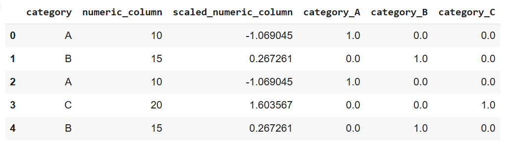
Output of code above
Data reduction simplifies the dataset by reducing the number of features or records while preserving the essential information. This helps speed up analysis and model training without sacrificing accuracy.
Techniques for data reduction include:
And here’s how we implement dimensionality reduction in Python:
from sklearn.decomposition import PCA
from sklearn.feature_selection import SelectKBest, chi2

# Creating a manual dataset
data = pd.DataFrame({
    'feature1': [10, 20, 30, 40, 50],
    'feature2': [1, 2, 3, 4, 5],
    'feature3': [100, 200, 300, 400, 500],
    'target': [0, 1, 0, 1, 0]
	})

# Feature selection using SelectKBest
selector = SelectKBest(chi2, k=2)
selected_features = selector.fit_transform(data[['feature1', 'feature2', 'feature3']], data['target'])

# Printing selected features
print("Selected features (SelectKBest):")
print(selected_features)

# Dimensionality reduction using PCA
pca = PCA(n_components=2)
pca_data = pca.fit_transform(data[['feature1', 'feature2', 'feature3']])

# Printing PCA results
print("PCA reduced data:")
print(pca_data)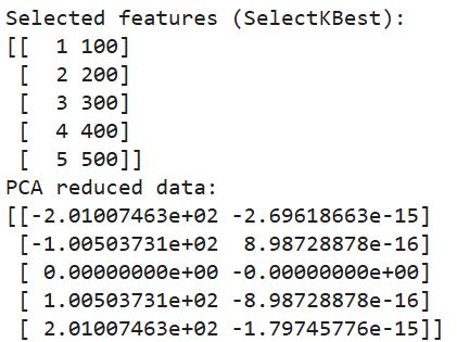
Output of code above
We’ve established that preprocessing raw data is essential to ensure it is well-suited for analysis or machine learning models. We’ve also covered the steps involved with the process.
In this section, we will explore various techniques for handling common issues during the preprocessing phase. Additionally, we will explore data augmentation, a useful technique for creating synthetic data in specific contexts like image or text datasets.
Missing data can negatively impact the performance of a machine learning model or analysis. There are several strategies to handle missing values effectively:
# Note: This is dummy code and not expected to run on its own
from sklearn.impute import SimpleImputer

imputer = SimpleImputer(strategy='mean')  # Replace 'mean' with 'median' or 'most_frequent' if needed
data['column_with_missing'] = imputer.fit_transform(data[['column_with_missing']])data.dropna(inplace=True) # Removes rows with any missing valuesOutliers are extreme values that deviate significantly from the rest of the data, which, like missing values, can distort analysis and model performance. Various techniques can be used to detect and handle outliers:
# Note: this is dummy code.
# It won’t work unless a data with a column named “column” is imported

from scipy import stats
z_scores = stats.zscore(data['column']) outliers = abs(z_scores) > 3 # Identifying outliersQ1 = data['column'].quantile(0.25)
Q3 = data['column'].quantile(0.75)
IQR = Q3 - Q1
outliers = (data['column'] < (Q1 - 1.5 * IQR)) | (data['column'] > (Q3 + 1.5 * IQR))When working with categorical data, encoding is necessary to convert categories into numerical representations that machine learning algorithms can process. Common encoding techniques include:
from sklearn.preprocessing import OneHotEncoder
encoder = OneHotEncoder(sparse_output=False)
encoded_data = encoder.fit_transform(data[['categorical_column']])from sklearn.preprocessing import LabelEncoder
le = LabelEncoder()
data['encoded_column'] = le.fit_transform(data['categorical_column'])from sklearn.preprocessing import OrdinalEncoder
oe = OrdinalEncoder(categories=[['low', 'medium', 'high']])
data['ordinal_column'] = oe.fit_transform(data[['ordinal_column']])Scaling and normalization ensure that numerical features are on a similar scale, which is particularly important for algorithms that rely on distance metrics (e.g., k-nearest neighbors, SVMs).
from sklearn.preprocessing import MinMaxScaler
scaler = MinMaxScaler()
data[['scaled_column']] = scaler.fit_transform(data[['numeric_column']])from sklearn.preprocessing import StandardScaler
scaler = StandardScaler()
data[['standardized_column']] = scaler.fit_transform(data[['numeric_column']])Data augmentation is a technique for artificially increasing the size of a dataset by creating new, synthetic examples. This is especially useful for image or text datasets in deep learning models, where large amounts of data are required for robust model performance.
from tensorflow.keras.preprocessing.image import ImageDataGenerator

datagen = ImageDataGenerator(
    rotation_range=40,
    width_shift_range=0.2,
    height_shift_range=0.2,
    shear_range=0.2,
    zoom_range=0.2,
    horizontal_flip=True,
    fill_mode='nearest')

augmented_images = datagen.flow_from_directory('image_directory', target_size=(150, 150))import nlpaug.augmenter.word as naw
# install nlpaug here: https://github.com/makcedward/nlpaug
aug = naw.SynonymAug(aug_src='wordnet')
augmented_text = aug.augment("This is a sample text for augmentation.")While you can implement data processing using pure Python code, powerful tools have been developed to handle various tasks and make the overall process more efficient. Here are a few examples:
There are quite a few specialized libraries for data preprocessing in Python. Here are 3 of the most popular:
import pandas as pd

# Load a sample dataset
data = pd.DataFrame({
    'name': ['John', 'Jane', 'Jack'],
    'age': [28, 31, 34]
})

print(data)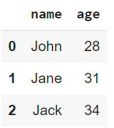
Output of code above
import numpy as np

# Create an array and perform element-wise operations
array = np.array([1, 2, 3, 4])
squared_array = np.square(array)

print(squared_array)![]()
Output of code above
from sklearn.preprocessing import StandardScaler

# Standardize data
data = [[10, 2], [15, 5], [20, 3]]
scaler = StandardScaler()
scaled_data = scaler.fit_transform(data)
print(scaled_data)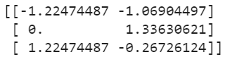
Output of code above
On-premise systems may not be able to handle large datasets effectively. In such situations, cloud platforms offer scalable, efficient solutions that enable you to process vast amounts of data across distributed systems.
Some cloud platform tools to consider include:
Automating the repetitive steps of preprocessing data can save time and reduce errors – especially when dealing with machine learning models and large datasets. Here are some tools that offer built-in preprocessing pipelines:
from sklearn.pipeline import Pipeline
from sklearn.preprocessing import StandardScaler, OneHotEncoder
from sklearn.impute import SimpleImputer
from sklearn.compose import ColumnTransformer

# Example Pipeline combining different preprocessing tasks
numeric_transformer = Pipeline(steps=[
    ('imputer', SimpleImputer(strategy='mean')),
    ('scaler', StandardScaler())
])

categorical_transformer = Pipeline(steps=[
    ('imputer', SimpleImputer(strategy='most_frequent')),
    ('encoder', OneHotEncoder())
])

preprocessor = ColumnTransformer(transformers=[
    ('num', numeric_transformer, ['age']),
    ('cat', categorical_transformer, ['category'])
])

preprocessed_data = preprocessor.fit_transform(data)It’s essential to follow the best practices to maximize the effectiveness of your preprocessing efforts. That said, below are some practices I’d encourage you to consider:
Before you dive into preprocessing, it’s important to understand the dataset thoroughly. Conduct exploratory data analysis to identify the structure of the data at hand. What you want to understand specifically are:
Without first understanding the dataset’s characteristics, it’s quite likely you may apply incorrect preprocessing methods, which will distort the data.
Preprocessing often involves repetitive tasks. Automating these tasks by building pipelines ensures consistency and efficiency and reduces the odds of manual errors. To streamline workflows, leverage pipelines in tools like scikit-learn or cloud-based platforms.
Clear documentation helps achieve two objectives:
Every decision, transformation, or filtering step should be recorded, including its reasoning. This will significantly enhance collaboration among team members and help you pick up projects where you left off.
Data preprocessing is not a one-time task – it should be an iterative process. As models evolve and provide feedback on their performance, use this information to revisit and refine preprocessing steps, as it can lead to better results. For instance, feature engineering may reveal new useful features, or tuning outlier handling may improve model accuracy – use this feedback to update your preprocessing steps.
Data preprocessing plays a critical role in the success of any data project. Proper preprocessing ensures that raw data is transformed into a clean, structured format, which helps models and analyses yield more accurate, meaningful insights.
In this article, I’ve shared various techniques to help implement data preprocessing. Still, the most important thing to note is that this process is not a one-time effort but an iterative process! Continuous refinement leads to improved model performance and better decision-making. A well-prepared dataset sets the foundation for any successful data AI initiative.
To continue your learning, I recommend checking out the following excellent resources:
Learn more about data engineering with these courses!
Course
Course
Course
Tutorial
Rajesh Kumar
Tutorial
Sejal Jaiswal
Tutorial
Moez Ali
Tutorial
Srujana Maddula
Tutorial
DataCamp Team
Tutorial
Amberle McKee