How to Freeze Multiple Rows in Excel

By default, the “Freeze Top Row” option in Excel only locks the very first row in place. Depending on your case, this may not be useful. Excel does offer the option to freeze multiple rows, but it takes an extra step.

If you are getting started in Excel, our Introduction to Excel course covers skills like navigating the interface, understanding data formats, and working with basic functions. Also, I find the Excel Formulas Cheat Sheet, which you can download, as a helpful reference because it has all the most common Excel functions.

The Right Way to Freeze Multiple Rows

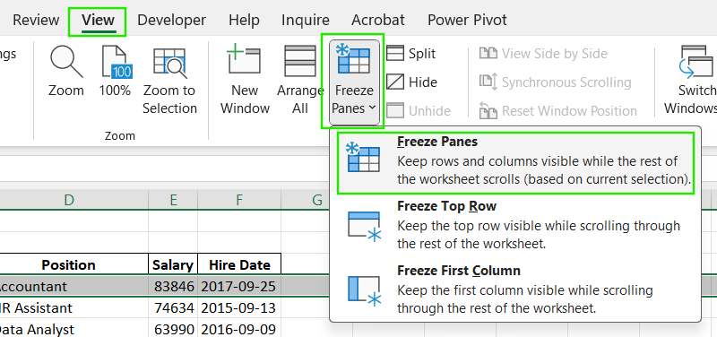
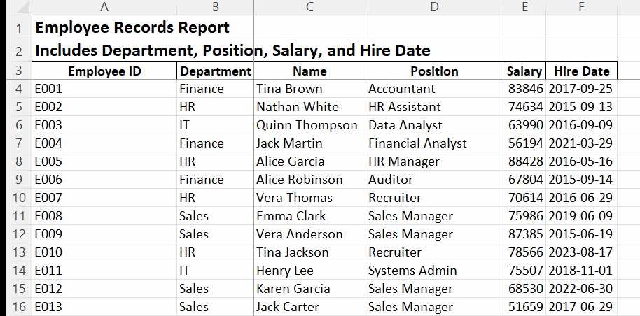
To freeze multiple rows in Excel, you use the Freeze Panes command. This command is more flexible than the "Freeze Top Row" option because it freezes all rows above the cell you've selected. Use the steps below:

• Select the row immediately below the last one you want to freeze. For example, to freeze rows 1, 2, and 3, you must select row 4. The entire row should be selected, not just a single cell.
• Go to the View tab on the ribbon, then select the Freeze Panes dropdown menu.
• Select Freeze Panes from the options.

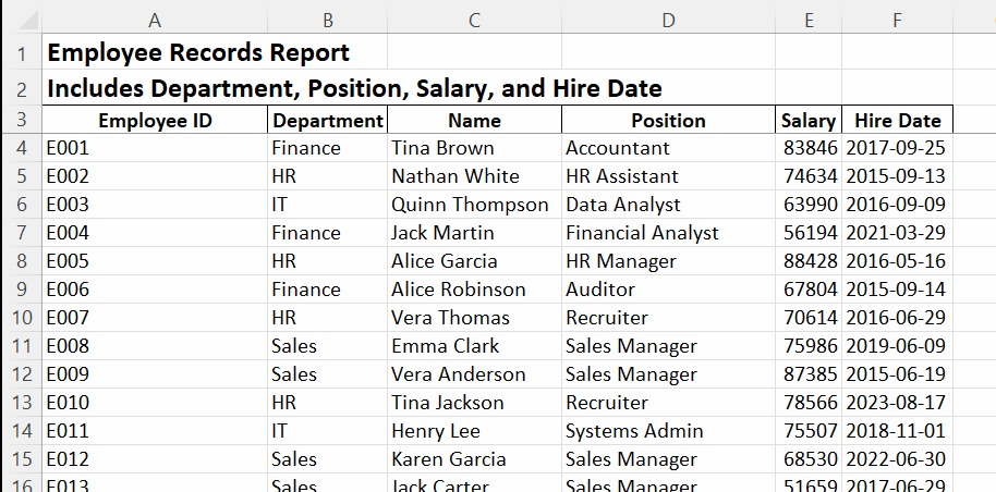
You will note that a thin gray line will appear below row 3, indicating that the top three rows are now frozen.

I recommend taking our Data Preparation in Excel course to learn more about cleaning and organizing your rows and columns. 

What You Can’t Do When Freezing Rows

When freezing rows in Excel, it’s important to understand these common limitations and misconceptions:

• You can’t multi-select rows to freeze them. The Freeze Panes option only works on the single row you have selected. If you select multiple rows and try to apply the command, it will not work as intended.
• You can’t freeze non-contiguous rows. For example, you cannot freeze row 1 and row 5 while leaving rows 2, 3, and 4 unfrozen. The Freeze Panes command always freezes a continuous block of rows from the very top of the spreadsheet down to your selected row.
• The “Freeze Top Row” option only locks row 1. This is a separate, dedicated command within the Freeze Panes dropdown menu.

Troubleshooting: When Freezing Multiple Rows Isn’t Working

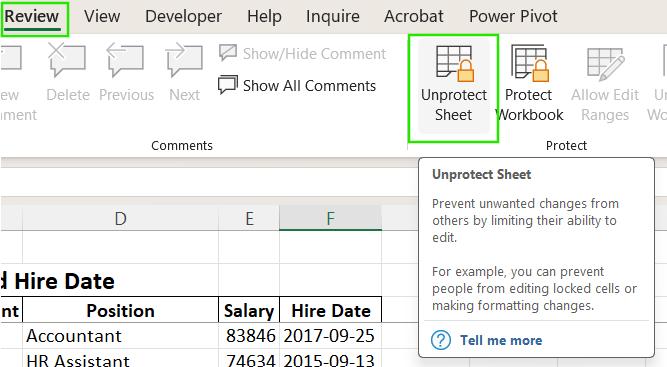
If you're having trouble freezing multiple rows in Excel, here are some common issues and their solutions:

• Freeze Panes option is grayed out: This is a common issue that often indicates you are not in the Normal View mode. To make this option active, switch to View > Workbook Views > Normal, and try again.

• The sheet is protected: If the worksheet is protected, many formatting and view options, including Freeze Panes, will be disabled to prevent unauthorized changes. To unprotect the sheet, go to the Review > Unprotect Sheet, then apply the freezing option.

• Sometimes you might accidentally select a column instead of a row before applying Freeze Panes. Remember to select the entire row below the rows you want to freeze.
• Some web-based or starter versions of Excel might have limited functionality compared to the full desktop version. Always check the features available in your specific version of Excel to confirm if the “Freeze Panes” option is available.

Check out our Excel Shortcuts Cheat Sheet, which you can download, to learn how to improve productivity by using shortcuts for different Excel features.

How to Freeze Rows and Columns at the Same Time

Sometimes, you may want to lock both the top rows and the left-side columns so your headers and labels stay visible as you scroll in any direction. In this case, you use the intersection logic, where you select a cell, and Excel freezes everything above and to the left of it. 

For example, let’s assume you want to freeze rows 1–3 and columns A–B:

• Select cell “C4”. This cell is immediately to the right of the last column you want to freeze (column B) and directly below the last row you want to freeze (row 3).

• Go to the View > Freeze Panes > Freeze Panes.

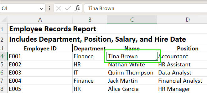
After you do this, a horizontal line will appear below row 3, and a vertical line will appear to the right of column B. Now rows 1 to 3 and columns A to B will remain visible as you scroll through your worksheet.

Excel Version Differences: Windows, Mac, and Office 365

The method of freezing panes is consistent across modern versions of Excel for Windows, Mac, and Microsoft 365. However, you might notice the following slight differences in the user interface or feature availability:

• Excel for Mac: The process is nearly identical to the Windows version. You can find the Freeze Panes command under the View tab and the steps to freeze multiple rows or columns remain the same.
• Excel 365: Users often mistakenly use the quick-access "Freeze Top Row" option when they need to use the more versatile "Freeze Panes" command to lock more than one row.
• Excel Starter: This is a lightweight version of Excel that comes pre-installed on some computers. It has limited features, and the Freeze Panes option may be unavailable.

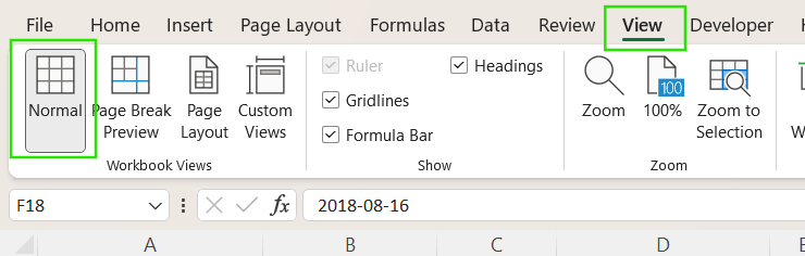
To avoid issues, always make sure you're in Normal View before you try to freeze panes. If you're not, the freezing options might not be available.

Pro Tips for Working with Frozen Rows

If you want to get the most out of Excel's freezing features, consider these advanced tips to enhance your workflow and data visualization.

• Use Freeze Panes with filters or slicers: This method keeps your header row visible so filters, dropdowns, or slicers remain accessible as you scroll.
• Avoid merged cells in frozen rows. Merged cells can behave inconsistently when frozen, making scrolling and alignment less consistent.
• Combine Freeze Panes with Split View: For side-by-side or top-bottom comparisons, you can use Split View with Freeze Panes. The Split View feature divides the worksheet into separate scrollable sections, each with its own scroll bar. This allows you to view different parts of a large sheet simultaneously.
• Add visual separators: To make frozen rows more distinct from the rest of your data, apply shading, bold fonts, or borders.

Conclusion

Freezing multiple rows in Excel comes down to choosing the right selection point. By selecting the row just below the ones you want to lock and using Freeze Panes, you can keep important headers and titles visible while you scroll. Whether you’re working with multi-level headers, dashboard layouts, or detailed datasets, this simple trick ensures you never lose context as you navigate your sheet.

If you want to advance your Excel skills, I recommend taking our Data Analysis in Excel course. This course will help you master advanced analytics and propel your career. I also recommend taking our Intermediate Power Query in Excel course to learn about data transformation and using the M language for creating dynamic functions.