Marginal Probability: Theory, Examples, and Applications

You're analyzing customer behavior for an e-commerce platform, and your manager asks: "What's the probability a customer churns, regardless of why?"

This question gets at something more specific than you might think. You're not asking about churn given a particular product category, or churn combined with payment method. You're asking about the baseline probability of a single event: customer churn, period.

That's marginal probability, and it's foundational to most probability calculations you'll encounter in data science.

What Is Marginal Probability?

As I introduced, marginal probability is the probability of a single event occurring, irrespective of other variables or events. It's called "marginal" because when you write out joint probabilities in a table, these single-event probabilities appear in the margins (the row and column totals).

The notation is straightforward. For a discrete event A, we write P(A). Marginal probability often emerges from joint probability. If B is a discrete random variable and you know the joint probability of A occurring with each value of B, you can find the marginal probability by summing: P(A) = Σ_b P(A, B=b), where you sum over all possible values b that B can take. Marginal probability is what remains when you "sum over" or "integrate out" all other variables.

To understand this concept fully, you'll need some foundational terms. The sample space is the set of all possible outcomes. An event is any subset of the sample space. Joint probability P(A ∩ B) measures the likelihood of two events occurring together, while conditional probability P(A|B) measures the likelihood of A given that B has occurred.

I recommend checking out our Introduction to Probability Rules Cheat Sheet for a quick reference on these relationships. Marginal probability sits at the center of this probability ecosystem. It's the denominator in conditional probability calculations and the building block for Bayes' Theorem.

Marginal Probability from Tables and Distributions

Let's see how you actually calculate marginal probability from different data structures. The approach depends on whether you're working with discrete or continuous variables.

Discrete case (contingency tables)

When working with categorical data, marginal probabilities appear naturally in contingency tables. Suppose you're analyzing customer purchase behavior across product categories (Electronics, Clothing, Books) and regions (North, South, East, West). Each cell contains the joint probability of a category-region combination. The row totals give you the marginal probability for each product category (P(Electronics), P(Clothing), P(Books)) regardless of region. Column totals give you marginal probabilities for each region.

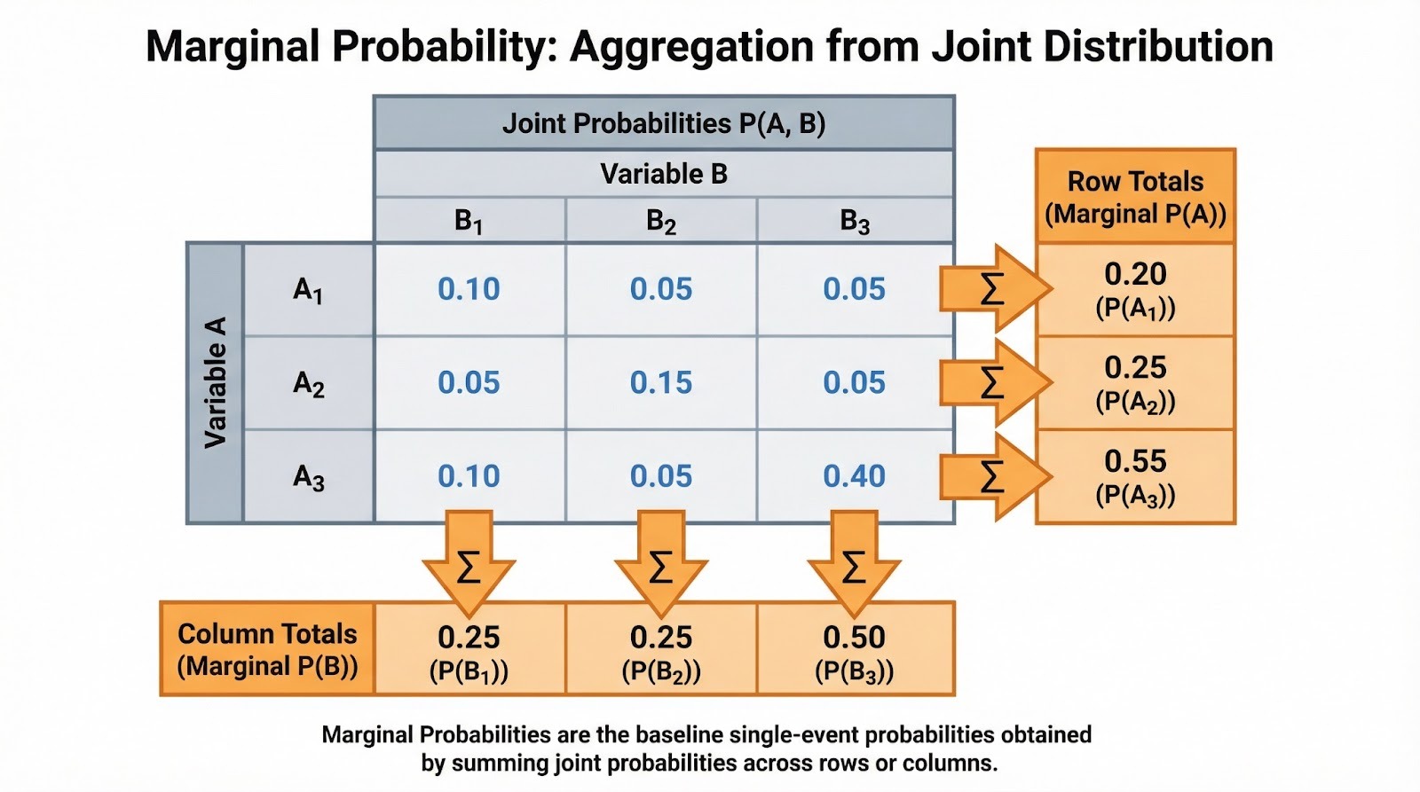
Summing joint probabilities to find marginal probabilities. Image by Author.

You'll often encounter these as normalized frequencies. If 500 out of 2,000 customers bought electronics, the marginal probability P(Electronics) = 500/2,000 = 0.25. This is the baseline rate before considering any other factors. When you're doing exploratory data analysis, I'd suggest calculating these marginals first. They help you understand your data's basic structure before diving into conditional relationships.

Continuous case

For continuous random variables, marginal probability becomes a marginal probability density function (PDF). If you have two continuous variables X and Y with a joint PDF, the marginal PDF of X is found by integrating over all values of Y.

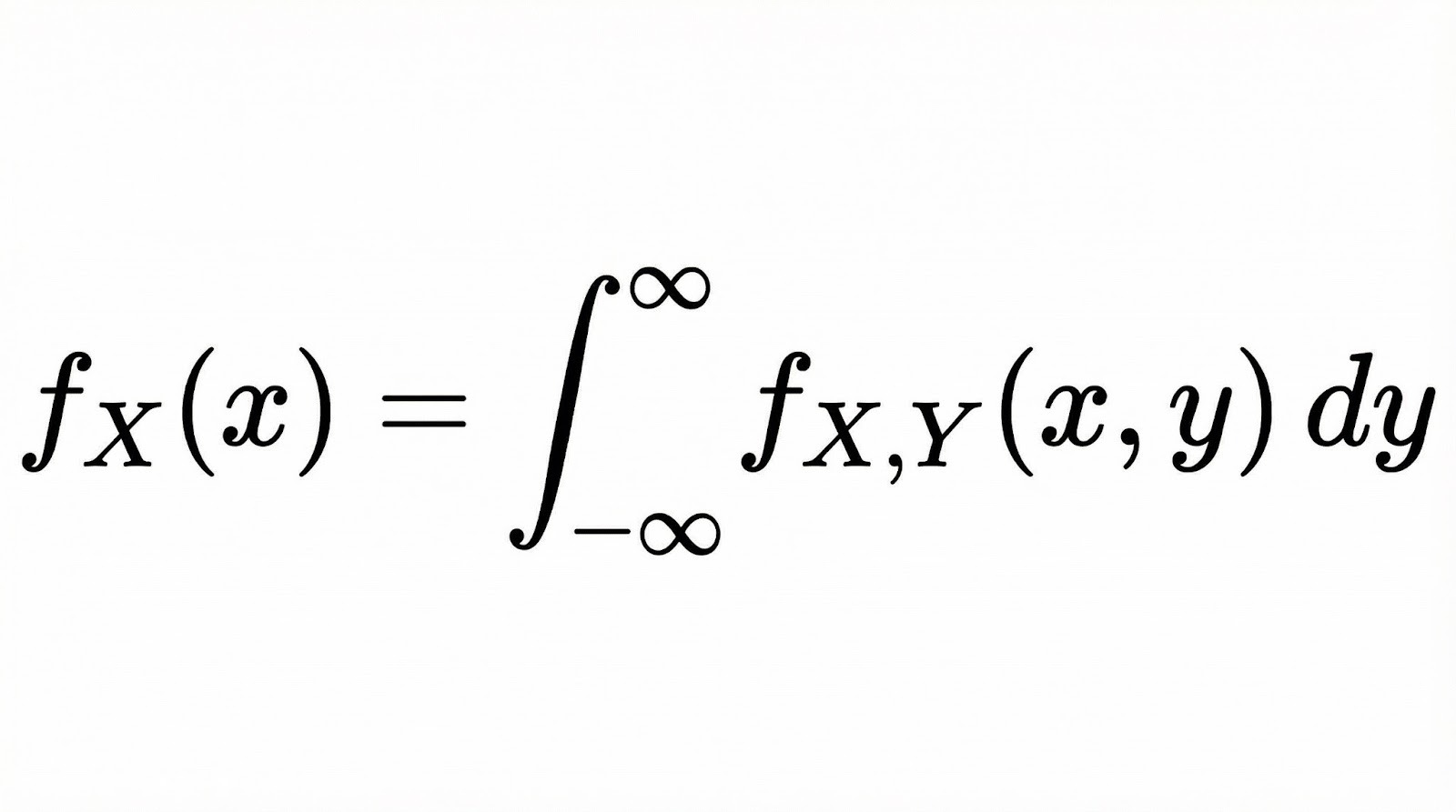
Conceptually, integration here does the same thing as summation in the discrete case. It "collapses" the joint distribution down to a single dimension by accounting for all possibilities of the other variable.

Think of it as slicing through a 3D surface (the joint distribution) and looking at the area under the curve along one axis. Our Fundamentals of Bayesian Data Analysis in R course covers these concepts in depth when working with continuous distributions.

Relationship Between Marginal, Joint, and Conditional Probability

Let's examine how marginal probability connects to the other probability types you'll work with regularly.

These three types of probability form a connected system, and marginal probability is often the glue holding them together. From joint probability, you get marginals by summing or integrating. From joint and marginal probabilities, you calculate conditionals using P(A|B) = P(A ∩ B) / P(B). Notice that marginal probability P(B) is the denominator. It normalizes the joint probability to give you the conditional.

This matters in practice because when you're interpreting conditional probabilities, you need the marginal as context. A 90% probability of disease given positive test results sounds alarming, but if the marginal probability of disease is only 1%, the actual probability after a positive test might be much lower than you'd expect.

This shows up everywhere in Bayesian inference. A prior is your belief about a parameter before seeing any data. The marginal likelihood (also called the evidence), P(Data), is the normalization term in Bayes’ theorem that turns “prior × likelihood” into a proper posterior probability. Our Bayesian Data Analysis in Python course explores these connections through practical modeling exercises.

Worked Examples of Marginal Probability

Let's work through both classical probability problems and real-world scenarios.

Classical examples

Let's start with dice. If you roll two dice, what's the probability the first die shows a 4, regardless of the second die's value?

The sample space has 36 equally likely outcomes. Six of these have a 4 on the first die: (4,1), (4,2), (4,3), (4,4), (4,5), (4,6). So P(First die = 4) = 6/36 = 1/6. Notice we didn't condition on anything about the second die. We simply counted all outcomes where the first die is 4.

Here's another classic example. Drawing from a standard 52-card deck, what's the probability of drawing a heart, regardless of rank? There are 13 hearts and 52 total cards, so P(Heart) = 13/52 = 1/4. This marginal probability aggregates across all ranks (Ace through King), giving you the unconditional probability of the suit.

Real-world examples

Medical screening provides a compelling real-world application. Suppose you're analyzing disease prevalence in a population. The marginal probability P(Disease) represents the baseline disease rate before considering any diagnostic test results. If 2% of the population has the disease, P(Disease) = 0.02. This marginal probability is essential for interpreting test accuracy. A test with 95% sensitivity still produces many false positives when the disease is rare.

In digital marketing, you might ask: What's the probability a user converts, regardless of traffic source? If you have data on conversions from organic search, paid ads, social media, and email, the marginal probability P(Conversion) sums across all sources. This baseline conversion rate helps you assess whether specific traffic sources perform above or below average.

Similarly, in finance, you might calculate the marginal probability of a market decline regardless of interest rate levels. This gives you the unconditional risk before layering in macroeconomic factors.

Marginal Probability in Data Science and Machine Learning

Let's explore how marginal probability appears throughout the data science workflow.

Exploratory data analysis (EDA)

When you first encounter a dataset, calculating marginal probabilities helps you understand baseline event rates. In a fraud detection dataset, P(Fraud) tells you the class balance before you examine any features. This immediately reveals whether you're dealing with a severely imbalanced problem where fraud occurs in only 0.1% of transactions.

Marginal distributions for individual features also guide your analysis. If you're building a model to predict customer churn, I'd recommend examining P(Churn), P(High-value customer), and P(Recent activity) separately. This provides context before you explore their joint relationships.

Predictive modeling

Naive Bayes classifiers rely explicitly on marginal probabilities as class priors. When classifying a document as spam or not spam, P(Spam) is your prior belief before seeing any words in the document. The algorithm then updates this marginal probability based on conditional feature probabilities.

Marginal feature distributions also matter in feature engineering and model diagnostics. If a feature's marginal distribution is highly skewed, you might apply transformations like log scaling or Box-Cox to make it more symmetric. 

Shifts between datasets are equally important. For example, if your training set has P(Class A)=0.9 but your test set has P(Class A)=0.5, your predicted probabilities and performance metrics can change a lot, and you may need a different decision threshold. This happens because the model learned under one base rate, but it’s being evaluated under another.

Checking marginal distributions before training helps you catch these issues early and decide whether you need resampling, different evaluation metrics, recalibration, or separate models for different data segments.

Risk and decision-making

Expected value calculations require marginal probabilities. If you're deciding whether to launch a product, you need P(Success) as the marginal probability of success across all possible market conditions. Multiply this by the payoff for success, add it to P(Failure) times the cost of failure, and you have your expected value.

Probabilistic modeling

In Bayesian networks and graphical models, nodes represent variables with associated conditional probability distributions. Marginal distributions are obtained through inference by propagating probabilities through the network structure or by observing evidence and updating beliefs. Sampling methods like Markov Chain Monte Carlo approximate these marginals when exact calculation becomes intractable. Our Bayesian Modeling with RJAGS course demonstrates these methods in practice.

What People Get Wrong About Marginal Probability

Here are the mistakes that trip up even experienced practitioners.

Confusing marginal with conditional probability

This is probably the most common mistake, and it's surprisingly intuitive to make. Imagine you take a medical test with 95% sensitivity and 90% specificity. You test positive. Most people immediately think: "The test catches 95% of cases, so I probably have the disease."

But that reasoning skips a critical piece of information: how common is the disease in the first place? If only 1% of people have it (the marginal probability), then when you test 10,000 people, you'll get about 95 true positives but 990 false positives. That means most positive results are false alarms. Your actual probability after testing positive is only about 9%, not 95%.

The confusion happens because people focus on the test's sensitivity (95%) and forget about the baseline rate (1% prevalence). The marginal probability P(Disease) = 0.01 and the conditional probability P(Disease | Positive test) = 0.09 are completely different quantities, but our intuition wants to treat them the same.

Ignoring marginals when interpreting conditionals

Even when people correctly distinguish marginal from conditional probabilities, they often ignore the marginal when interpreting conditionals. You might see a news headline: "Study finds 80% of successful entrepreneurs started before age 30." That's P(Started before 30 | Successful entrepreneur) = 0.8. But without knowing P(Started before 30) for all entrepreneurs, you can't assess whether starting young actually predicts success.

This leads to flawed decision-making. If 90% of all entrepreneurs start before 30, then successful entrepreneurs don't start young at unusual rates. They're just following the general pattern. The conditional probability means little without the marginal baseline for comparison.

Base rate fallacy

The base rate fallacy occurs when people overweight conditional evidence while ignoring marginal probabilities (base rates).

Here's a common data science example: You're building a binary classifier on an imbalanced dataset. The positive class (what you're trying to predict) occurs in only 5% of your data. You build a model and achieve 95% accuracy. That sounds great, right?

Not really. If you built a "dumb" model that just predicts the negative class every single time, it would also get 95% accuracy (because 95% of the data is negative). Your fancy model isn't actually doing much better than always guessing "no."

The mistake is looking at the 95% accuracy number in isolation without considering the base rate (5% positive class). When classes are imbalanced, accuracy becomes a misleading metric. You need to check precision, recall, or F1-score to see if your model actually learned anything useful.

Understanding marginals helps you choose the right evaluation metrics for imbalanced problems.

Advanced Topics and Extensions

In high-dimensional models with dozens or hundreds of variables, computing marginal distributions exactly is often impossible. The number of possible combinations grows rapidly, and the required sums or integrals become intractable.

To handle this, practitioners use approximate inference methods:

• Sampling methods (like Markov Chain Monte Carlo, MCMC) generate many samples from the model’s distribution. You can then estimate marginal probabilities by looking at how often events occur in those samples.

• Variational inference takes a different approach: it replaces a hard-to-compute distribution with a simpler one and optimizes it to be as close as possible, making marginal estimates often faster in large models.

Modern tools like Python's scipy.stats for probability distributions, pandas for contingency tables, and R's table() and dplyr for empirical marginals make these calculations accessible. For database-stored data, SQL's GROUP BY clause computes empirical marginals efficiently from large datasets.

Conclusion

Before you can understand the relationship between variables, assess conditional evidence, or build Bayesian models, you need to grasp the unconditional probability of individual events. It's the baseline that makes everything else interpretable.

When you misunderstand marginals, you're vulnerable to analytical errors: confusing baseline rates with conditional probabilities, falling for the base rate fallacy, or building models that don't outperform naive baselines. Get marginals right, and you'll understand how conditional probability refines them, how Bayes' Theorem updates them with evidence, and how machine learning models learn from the patterns they reveal.