Geometric Distribution: A Complete Guide to Modeling First Success Events

How many job interviews might you need before landing your dream position? How many attempts does it take before a marketing campaign generates its first sale? The geometric distribution answers these "waiting time" questions by modeling the number of trials needed until the first success occurs.

This guide covers the geometric distribution's mathematical foundation, its distinctive properties, and practical applications that make it valuable for people who work with sequential trial scenarios. For a refresher on probability distributions, consider taking our Introduction to Statistics course. 

What Is the Geometric Distribution?

The geometric distribution is a discrete probability distribution that models the number of independent Bernoulli trials required to achieve the first success. Each trial has the same probability of success, and trials are independent of each other.

This distribution comes in two common forms: one that counts the total number of trials until the first success (including the success), and another that counts only the number of failures before the first success. Both forms are widely used depending on the specific application context. Throughout this guide, we'll use the first form, counting the total number of trials until the first success, where X can take values 1, 2, 3, and so on.

Understanding the Geometric Distribution

Let's examine the mathematical structure and characteristics that define this distribution.

Fundamental definition and probability structure

The geometric distribution requires three key conditions: independent trials, identical probability of success across all trials, and a fixed probability p where 0 < p ≤ 1. The standard notation uses p for the probability of success and q = 1-p for the probability of failure.

The probability mass function (PMF) for the number of trials X until first success is: 

This formula calculates the probability of experiencing exactly k-1 failures followed by one success. For example, if p = 0.3, the probability of success on the third trial is P(X = 3) = (0.7)² × 0.3 = 0.147.

Cumulative probabilities and distribution function

The cumulative distribution function (CDF) gives us:

This represents the probability of achieving success within k trials. Using our example where p = 0.3, let's calculate the CDF for the first few values:

• F(1) = P(X ≤ 1) = 1 - (0.7)¹ = 0.3
• F(2) = P(X ≤ 2) = 1 - (0.7)² = 1 - 0.49 = 0.51
• F(3) = P(X ≤ 3) = 1 - (0.7)³ = 1 - 0.343 = 0.657

This shows there's a 30% chance of success on the first trial, a 51% chance of success within the first two trials, and a 65.7% chance of success within the first three trials.

Graphing the geometric distribution

The geometric distribution's visual patterns show key insights about "waiting time" scenarios. These graphs demonstrate how probability concentrates in early trials and decreases exponentially, making the distribution useful for modeling situations where success is more likely sooner rather than later.

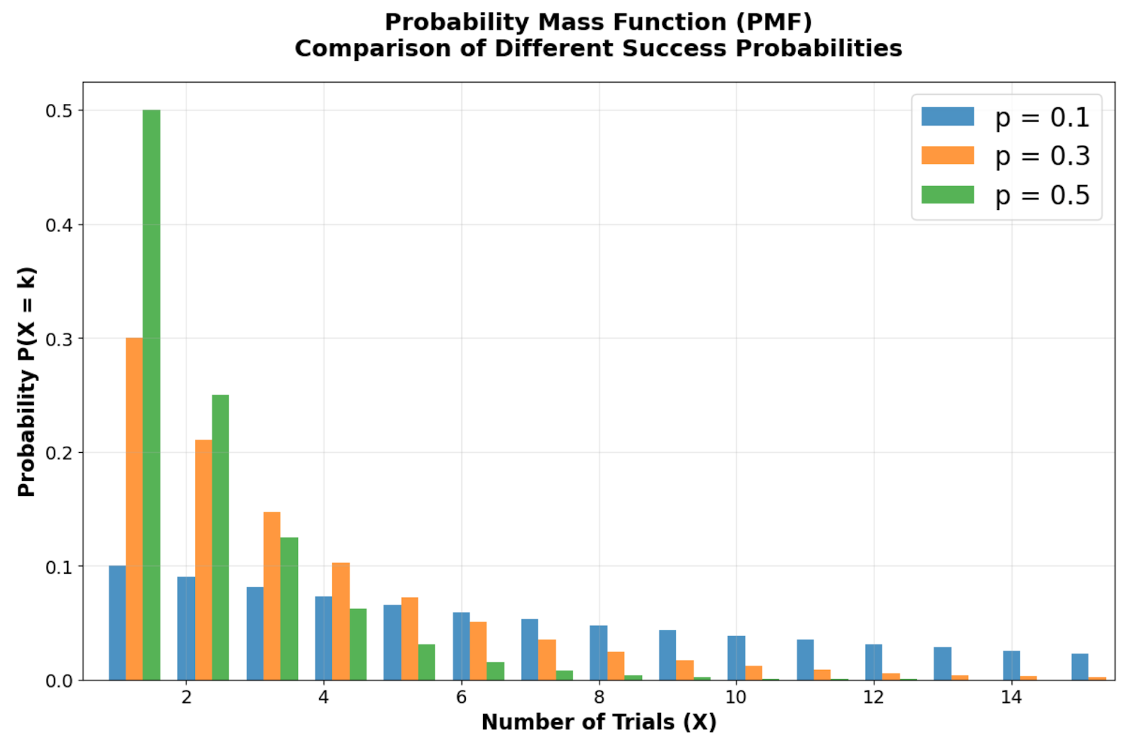
Probability Mass Function comparison showing how different success probabilities (p = 0.1, 0.3, 0.5) affect the distribution shape. Image by Author

Looking at the probability mass function comparison across different success probabilities, you can see the geometric distribution's distinctive right-skewed shape with its mode always at X = 1 (the first trial). Notice how the probability bars start highest at the first trial and decline geometrically for each subsequent trial. As the success probability p decreases, the distribution becomes more spread out, reflecting longer expected waiting times. For instance, with p = 0.1, there's only a 10% chance of immediate success, creating a more pronounced right tail compared to p = 0.5.

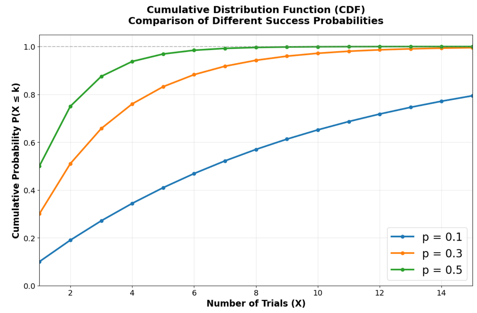
Cumulative Distribution Function showing how quickly different success probabilities approach certainty. Image by Author. 

The cumulative distribution function demonstrates how quickly the geometric distribution approaches certainty. Higher success probabilities create steeper curves that reach high cumulative probabilities within just a few trials. For example, with p = 0.5, there's approximately a 75% chance of success within the first two trials, while p = 0.1 requires significantly more trials to reach the same level of certainty.

Side-by-side comparison highlighting the exponential decay pattern in PMF and rapid approach to certainty in CDF. Image by Author. 

This exponential decay pattern explains why the geometric distribution works well for modeling scenarios where early success is more likely than prolonged waiting periods. The CDF's rapid ascent toward 1 shows why this distribution is effective for modeling processes where waiting times are short, making it valuable for quality control, customer conversion analysis, and reliability testing scenarios.

Creating your own geometric distribution visualizations

You can recreate these visualizations and explore different parameter values using Python's scipy and matplotlib libraries. Here's how to generate the key visual insights that highlight the geometric distribution's most important characteristics:

import numpy as np
import matplotlib.pyplot as plt
from scipy import stats

# Create side-by-side plots for PMF and CDF
fig, (ax1, ax2) = plt.subplots(1, 2, figsize=(16, 6))
fig.suptitle('Geometric Distribution: Key Visual Insights', fontsize=24, fontweight='bold')

# Simple PMF showing exponential decay (using p = 0.3)
x_simple = np.arange(1, 11)
pmf_simple = stats.geom.pmf(x_simple, 0.3)

ax1.bar(x_simple, pmf_simple, alpha=0.8, color='steelblue', edgecolor='black', linewidth=1)
ax1.set_title('PMF: Exponential Decay Pattern', fontsize=18, fontweight='bold', pad=15)
ax1.set_xlabel('Number of Trials (X)', fontsize=17, fontweight='bold')
ax1.set_ylabel('Probability', fontsize=14, fontweight='bold')
ax1.grid(True, alpha=0.3)
ax1.tick_params(axis='both', which='major', labelsize=14)

# Simple CDF showing approach to 1
cdf_simple = stats.geom.cdf(x_simple, 0.3)

ax2.plot(x_simple, cdf_simple, 'o-', linewidth=4, markersize=8, color='darkgreen')
ax2.set_title('CDF: Rapid Approach to Certainty', fontsize=18, fontweight='bold', pad=15)
ax2.set_xlabel('Number of Trials (X)', fontsize=17, fontweight='bold')
ax2.set_ylabel('Cumulative Probability', fontsize=14, fontweight='bold')
ax2.grid(True, alpha=0.3)
ax2.set_ylim(0, 1.05)
ax2.tick_params(axis='both', which='major', labelsize=14)

plt.tight_layout()
plt.show()	

This code creates a focused visualization that emphasizes the geometric distribution's two most important visual characteristics. The left panel shows how probabilities decay exponentially from the first trial, while the right panel demonstrates the rapid accumulation of probability mass in the CDF.

Try changing the success probability from 0.3 to different values like 0.1 or 0.7 to see how the distribution shape changes. Lower probabilities create flatter PMF curves and slower-rising CDFs, while higher probabilities create steeper declines and faster approaches to certainty.

Memoryless Property of Geometric Distribution

The geometric distribution has a unique characteristic that sets it apart from most other discrete distributions.

The memoryless property

The memoryless property states that P(X > s + t | X > s) = P(X > t) for any positive integers s and t. This means the probability of needing additional trials doesn't depend on how many unsuccessful trials have already occurred.

Mathematically, this property emerges because P(X > k) = (1-p)^k, making the conditional probability calculation straightforward. In practical terms, if you've already had five unsuccessful job interviews, the probability distribution for future interviews remains identical to when you started—past failures don't influence future probabilities.

Relationship to Bernoulli trials and experiments

Each trial in a geometric experiment represents an independent Bernoulli trial with constant success probability p. The geometric distribution models the sequence of these trials until the first success, making it the discrete analog of "waiting time" problems.

This relationship explains why the geometric distribution appears frequently in quality control, where each item tested represents a Bernoulli trial, and we're interested in detecting the first defective item. The independence assumption ensures that finding defective items in early tests doesn't change the probability of finding defects in subsequent tests.

Contrast with continuous analogs

The exponential distribution serves as the continuous counterpart to the geometric distribution, both sharing the memoryless property. While the geometric distribution models discrete waiting times (number of trials), the exponential distribution models continuous waiting times (time until an event).

Both distributions find applications in reliability analysis and queuing theory. For example, the geometric distribution might model the number of server requests until the first failure, while the exponential distribution models the time until the next server failure occurs.

Mathematical Properties and Calculations

With the foundational concepts and unique properties in place, let's explore the mathematical tools that enable precise probability calculations and informed decision-making. These formulas and relationships will prove essential when applying the geometric distribution to real-world problems.

Mean, variance, and standard deviation

The expected value (mean) of the geometric distribution is: 

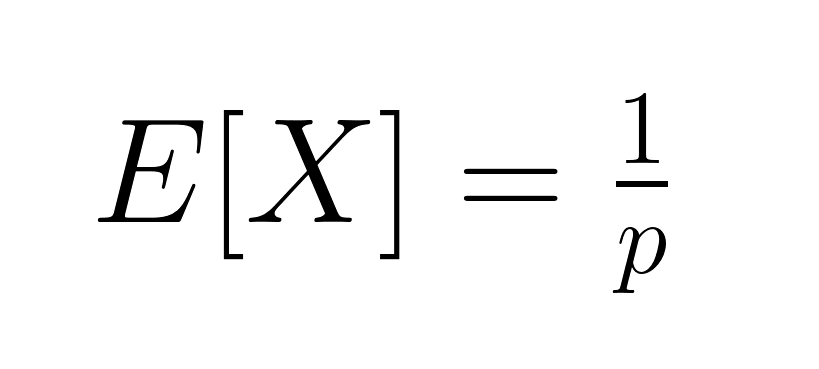
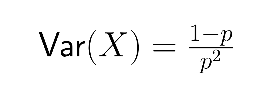
This represents the average number of trials needed for success. The variance equals:

The standard deviation is:

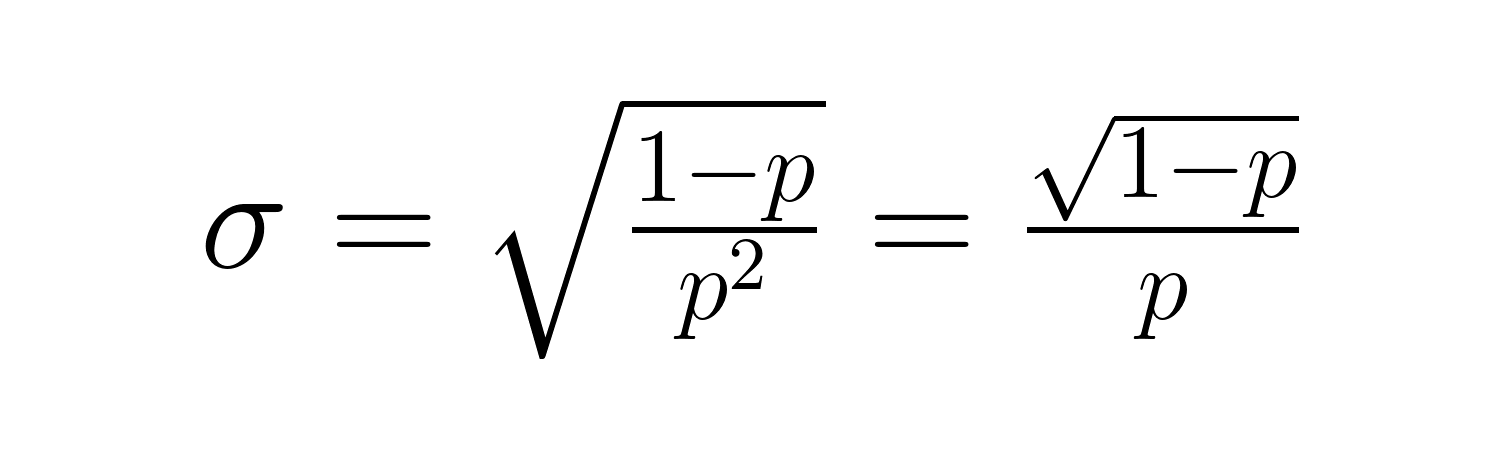
These formulas reveal important relationships: as p decreases, both the expected waiting time and variability increase significantly. For example, with p = 0.2, the expected number of trials is 5, but with p = 0.05, it jumps to 20 trials. The variance grows even more dramatically, from 20 to 380.

Moments and generating functions

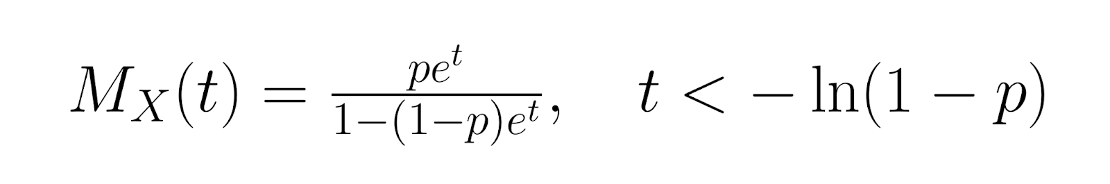
For more advanced analysis, the moment generating function (MGF) for the geometric distribution is:

The probability generating function (PGF) is:

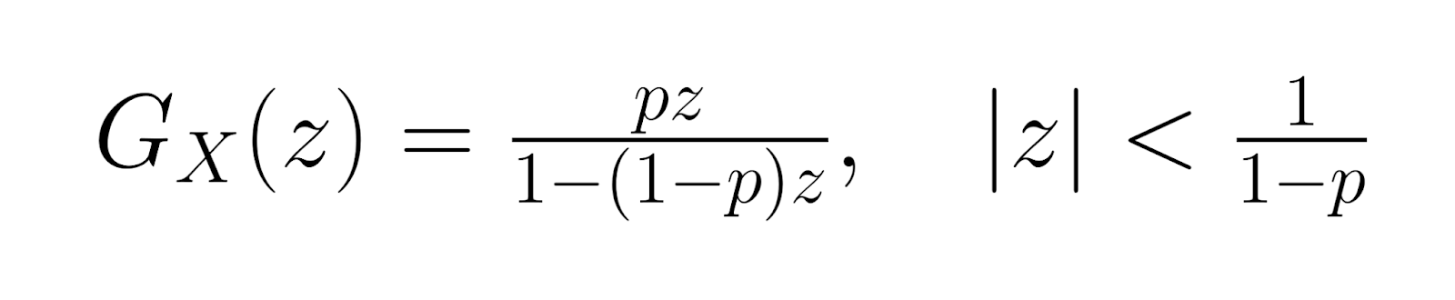
These generating functions help with advanced statistical analysis and provide alternative methods for deriving distribution properties. Higher-order moments can be calculated using derivatives of these functions, enabling comprehensive characterization of the distribution's shape and behavior.

Entropy and information measures (advanced)

Moving into more specialized territory, the entropy of the geometric distribution equals:

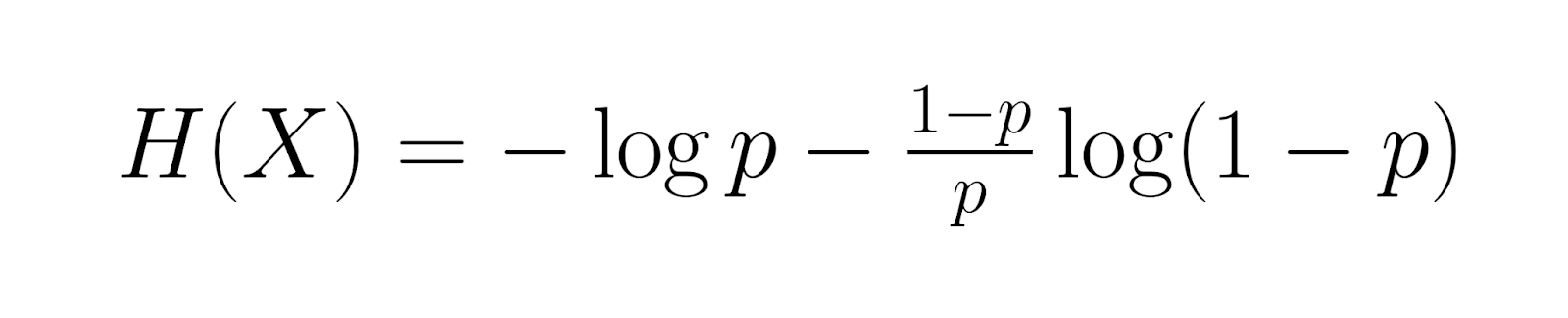
This measures the average information content. Fisher information, given by:

This quantifies the amount of information about parameter p contained in the data. These measures prove valuable in information theory applications and optimal experimental design, where understanding the information content helps determine appropriate sample sizes and estimation procedures.

Parameter Estimation Methods

Estimating the success probability p from observed data requires understanding different statistical approaches and their trade-offs.

Maximum likelihood estimation (MLE)

The maximum likelihood estimation approach works by finding the success probability that makes your observed data most likely to have occurred. To calculate this estimate, you divide the total number of success events by the sum of all trials across your observations. This estimator provides unbiased results and performs efficiently when working with large sample sizes.

Here's how this works in practice: if you observe success after 3, 7, 2, and 8 trials respectively, you would calculate the MLE by taking your 4 observations and dividing by the total of 20 trials (3+7+2+8), giving you an estimated success probability of 0.2 or 20%. The MLE approach maximizes the likelihood of observing the actual data you collected, making it the most statistically efficient method under standard conditions.

Method of moments

As an alternative approach, the method of moments estimator works by setting your sample average equal to the theoretical average of the geometric distribution. Since the theoretical mean equals one divided by the success probability, you can estimate the success probability by taking one divided by your sample mean. While this method offers computational simplicity compared to MLE, it can be less efficient statistically and may occasionally produce estimates that fall outside the valid probability range of zero to one.

Both methods produce similar results when working with large samples, but MLE generally offers superior statistical properties. The choice between methods often depends on computational constraints and the specific requirements of your analysis.

Bayesian estimation

When you have prior information available about the success probability, Bayesian estimation allows you to incorporate this knowledge through a prior probability distribution. The Beta distribution commonly serves as this prior because it works mathematically well with geometric distribution data. The Bayesian approach combines your prior beliefs with observed data to produce updated parameter estimates through what's called the posterior distribution.

The mathematical relationship creates an updated Beta distribution that incorporates both your prior knowledge and new observations. This approach works particularly well when you have limited data available or when you want to incorporate expert knowledge about the process being modeled. For example, if you know from industry experience that success rates typically fall within a certain range, you can incorporate this knowledge to improve your estimates even with small sample sizes.

Applications of Geometric Distribution

The geometric distribution finds extensive use across various industries and analytical contexts where modeling first success events provides insights.

Reliability engineering and quality control

Manufacturing processes often use geometric distribution to model defect detection and component failure analysis. Quality control inspectors can estimate the expected number of items to inspect before finding a defective unit, helping optimize inspection procedures and resource allocation.

For instance, if historical data shows a defect rate of 2%, the geometric distribution predicts an average of 50 items inspected before finding the first defect. This information helps determine appropriate batch sizes and inspection frequencies to maintain quality standards while minimizing costs.

Customer acquisition and network management

Marketing teams apply geometric distribution to model customer conversion processes, estimating how many contacts or advertisements are needed before achieving a sale. This analysis informs budget allocation and campaign strategy decisions.

In telecommunications, network engineers use geometric distribution to model packet transmission success rates and optimize retry mechanisms. Understanding the expected number of transmission attempts helps design efficient protocols and improve overall network performance.

Games, sports analytics, and additional real-world examples

Sports analysts use geometric distribution to model scoring events, such as the number of attempts needed for a basketball player to make their first three-point shot in a game. This analysis contributes to strategic decision-making and performance evaluation.

Gaming applications include modeling the number of attempts needed to achieve rare events or complete challenging levels. Online platforms use these insights to balance game difficulty and maintain player engagement through appropriate reward structures.

Solved sample problems and practice questions

Consider a scenario where a marketing campaign has a 15% conversion rate. To find the probability of getting the first conversion on the 5th contact: P(X = 5) = (0.85)⁴ × 0.15 = 0.0783 or about 7.83%.

For practice, calculate the probability that a quality control inspector finds the first defective item within the first 10 inspections, given a defect rate of 8%. Use the CDF formula: P(X ≤ 10) = 1 - (0.92)¹⁰ = 0.5656 or approximately 56.56%.

Limitations and Assumptions

Understanding when the geometric distribution applies appropriately requires recognizing its underlying assumptions and potential limitations.

The geometric distribution assumes independent trials with constant success probability, which may not hold in many real-world scenarios. For example, customer behavior often shows dependency—previous interactions can influence future conversion probabilities. Similarly, mechanical systems may experience wear that changes failure rates over time.

Violations of these assumptions can lead to inaccurate predictions and poor decision-making. Data practitioners should validate independence assumptions through statistical testing and consider alternative models when dependencies are detected. Common alternatives include the negative binomial distribution for overdispersed data or Markov chain models for dependent trials.

Conclusion

Understanding geometric distribution extends beyond theoretical knowledge—it enables you to make informed decisions about resource allocation, process optimization, and risk assessment. Whether you're designing quality control procedures or optimizing marketing campaigns, this distribution offers quantitative insights that drive better outcomes.

For continued learning, explore our Multivariate Probability Distributions in R course to understand how geometric distribution relates to other probability models, or dive deeper into estimation techniques with our Generalized Linear Models in R course for advanced modeling applications.