Conditional Probability: A Close Look

Imagine you're developing a spam detection system for email. Initially, you might flag an email as suspicious if it contains certain keywords. But what if you discover this email came from a trusted sender? Or what if it was sent at an unusual hour? Each piece of new information shifts the probability of the email being spam. This dynamic updating of probabilities based on new evidence lies at the heart of conditional probability, a concept that powers many modern data science applications, from email filtering to fraud detection. 

For those starting their journey with probability concepts, the Introduction to Probability Rules Cheat Sheet provides a helpful reference for core principles and formulas. The Introduction to Statistics course builds a solid foundation by exploring probability distributions and their properties, which form the basis for understanding how conditional probability works in practice. These resources offer a structured path to developing strong fundamentals in the concepts we'll explore in this article.

What is Conditional Probability?

Conditional probability measures how likely one event is to occur when we know another event has already taken place. When we receive new information about an event, we adjust our probability calculations accordingly.

To understand this concept, let's explore an example with playing cards. When you draw a card from a standard deck, there are 52 possible outcomes. If you want to draw a king, your initial probability is 4/52 (about 7.7%) since there are four kings in the deck. But what happens if someone tells you the card you drew is a face card? This new information changes everything - your probability of having a king is now much higher at 4/12 (about 33.3%), since there are only twelve face cards total.

This relationship between probabilities has a precise mathematical definition:

This formula helps us calculate conditional probability, where:

• P(A|B) represents the probability of event A occurring, given that event B has occurred. This is read as "the probability of A given B."
• P(A∩B) represents the joint probability, or the probability of both events A and B occurring together. This is read as "the probability of A intersection B."
• P(B) represents the probability of event B occurring.

In our card example:

• Event A is "drawing a King"
• Event B is "drawing a face card"
• P(A|B) = 4/12 (probability of getting a king, given we have a face card)
• P(A∩B) = 4/52 (probability of drawing a king, which is always a face card)
• P(B) = 12/52 (probability of drawing any face card)

To better understand how conditional probability works in practice, we can use a tree diagram. Tree diagrams are particularly helpful because they show how each piece of new information changes our probabilities:

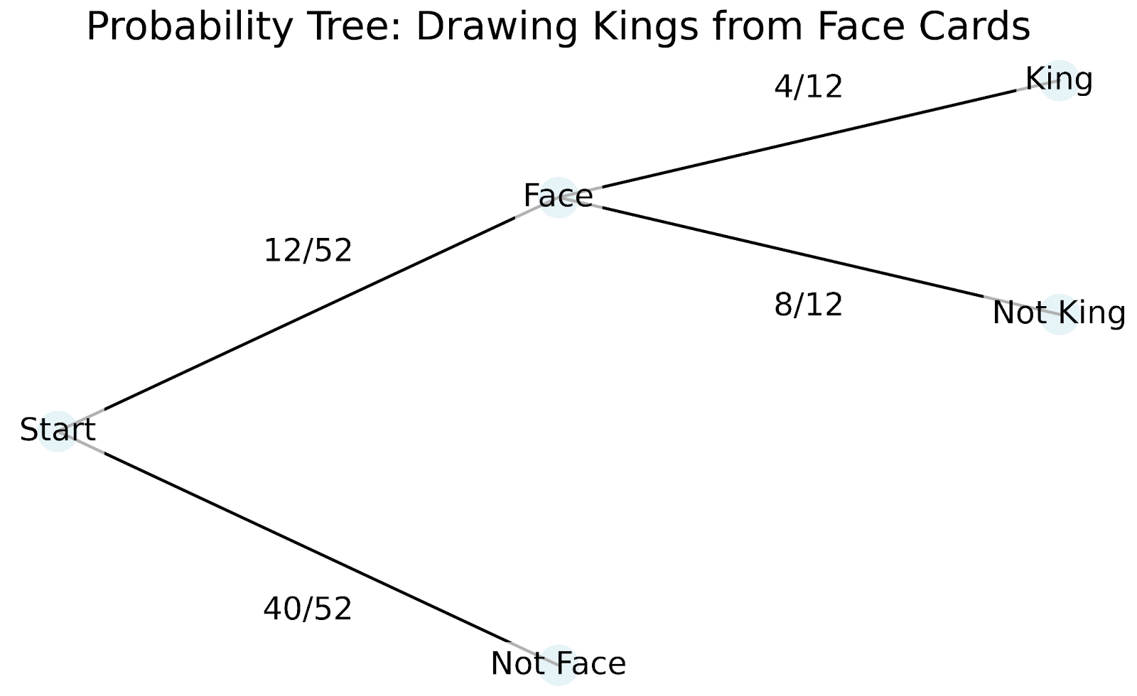
Let's walk through how this tree diagram works:

1. We start at the root (leftmost point) with all 52 cards.
2. The first branches show our first piece of information - is it a face card or not?
3. If we follow the face card branch, it splits again based on our second piece of information - is it a king?

The tree diagram helps us understand several key concepts in conditional probability:

• Sample Space: This is all possible outcomes in our scenario. The initial sample space is 52 cards, but it gets "reduced" to 12 cards once we know we have a face card.
• Events: These are specific outcomes we're interested in, like "drawing a face card" or "drawing a king." The branches in our tree represent different events.
• Joint Probability: This is the probability of multiple events occurring together. In our tree, we can find this by multiplying probabilities along a path. For example, the probability of drawing a king AND it being a face card is (12/52) × (4/12) = 4/52.
• Marginal (Unconditional) Probability: This is the probability of an event occurring without considering any other information. In our example, this is like the initial 4/52 probability of drawing a king before we know anything else about the card.

The beauty of conditional probability is that it allows us to update our probabilities as we gain new information. Just as we adjusted our probability of having a king from 7.7% to 33.3% when we learned we had a face card, conditional probability gives us a formal way to recalculate probabilities based on new evidence.

The Conditional Probability Formula

The mathematical structure of conditional probability provides us with tools to analyze complex scenarios involving multiple events. Let's explore the key properties.

Key properties of conditional probability

These mathematical properties help us solve complex problems more efficiently:

1. Independence property

When two events A and B are independent we know that the occurrence of one doesn't affect the probability of the other. Mathematically, this is: P(A|B) = P(A), which is read as: "the probability of A given B equals the probability of A."

For example, if we roll a die and flip a coin, getting heads on the coin doesn't change the probability of rolling a six. The formula shows us: P(Six|Heads) = P(Six) = 1/6

2. Complement rule

For any event A given condition B, the probabilities of A and its complement A' (read as "A prime") must sum to 1. Mathematically, this is: P(A|B) + P(A'|B) = 1, which is read as: “The probability of A given B plus the probability of A complement given B equals 1."

In our earlier card example: P(King|Face Card) + P(Not King|Face Card) = 4/12 + 8/12 = 1

The multiplication rule and chain rule

The multiplication rule links joint probabilities with conditional probabilities: P(A ∩ B) = P(A|B) × P(B). We say, "The probability of A intersection B equals the probability of A given B times the probability of B."

This extends to multiple events through the chain rule. For three events A, B, and C: P(A ∩ B ∩ C) = P(A|B ∩ C) × P(B|C) × P(C). That is, "The probability of A intersection B intersection C equals the probability of A given B intersection C times the probability of B given C times the probability of C."

Let's see this in action with a card drawing sequence:

1. Drawing a king (K)
2. From remaining cards, drawing a queen (Q)
3. From remaining cards, drawing an ace (A)

P(K ∩ Q ∩ A) = P(A|K ∩ Q) × P(Q|K) × P(K) = (4/50) × (4/51) × (4/52)

The chain rule becomes particularly valuable in machine learning, especially in Bayesian networks where we need to model complex dependencies between multiple variables. When analyzing data, we often encounter situations where events follow a natural sequence, and the chain rule helps us decompose these complex scenarios into simpler, more manageable calculations.

Examples to Illustrate Conditional Probability

Let's review two of the most common examples and think also about how conditional probability might show up in your work.

Classical examples

These two examples are very common and are worth studying, especially if you are interviewing:

Dice rolls: Understanding reduced sample spaces

When we roll a die, our sample space starts with six possibilities: {1, 2, 3, 4, 5, 6}. Learning partial information about the roll changes our probability calculations in a specific way. Let's see how:

Initial probability of rolling a 6: P(6) = 1/6

If we learn the roll was even, our sample space reduces to {2, 4, 6}: P(6 | even) = 1/3

Marbles: Sequential dependencies

A bag contains 5 blue marbles and 3 red marbles. When we draw marbles without replacement, each draw affects the probabilities of subsequent draws.

First draw - probability of blue: P(blue₁) = 5/8

Second draw, given first was blue: P(blue₂ | blue₁) = 4/7

This example complements our earlier card example by highlighting sequential dependencies.

Real-world examples

Medical testing: Evaluating test accuracy

Medical tests provide a perfect application of conditional probability in assessing test accuracy. For any diagnostic test, we need to understand four key conditional probabilities:

1. P(T+ | D+): Probability of a positive test given the patient has the disease (sensitivity) 
2. P(T- | D-): Probability of a negative test given the patient doesn't have the disease (specificity) 
3. P(T+ | D-): Probability of a positive test given the patient doesn't have the disease (false positive rate) 
4. P(T- | D+): Probability of a negative test given the patient has the disease (false negative rate)

When evaluating this test's performance, medical professionals use these conditional probabilities to:

1. Compare test accuracy across different patient populations
2. Determine when multiple tests might be needed
3. Set appropriate thresholds for positive/negative results

For instance, if we test 1000 patients and get 100 positive results, we can use these conditional probabilities to estimate how many are true positives versus false positives. This analysis helps medical professionals balance the risks of missing a diagnosis against the costs and anxiety of false alarms.

Financial risk assessment

Investment firms use conditional probability to evaluate market risks. Consider a portfolio manager tracking market volatility:

Daily market volatility can be Low (L), Medium (M), or High (H).

Historical data shows: 

• P(H tomorrow | H today) = 0.70 
• P(M tomorrow | H today) = 0.25 
• P(L tomorrow | H today) = 0.05

This information helps managers:

• Adjust portfolio allocations based on current market conditions
• Set risk thresholds for automated trading systems
• Develop contingency plans for periods of sustained high volatility

Conditional Probability and Bayes' Theorem

Our exploration of medical testing highlighted an important distinction: The probability of having a disease given a positive test differs from the probability of testing positive given the disease. Bayes' Theorem provides a formal framework for navigating this relationship, allowing us to update our probability estimates as new evidence emerges.

Understanding Bayes' Theorem

Bayes' Theorem expresses the relationship between two conditional probabilities: P(A|B) = [P(B|A) × P(A)] / P(B). We read this equation this way: "The probability of A given B equals the probability of B given A times the probability of A, divided by the probability of B."

Each component plays a role:

• P(A): The prior probability - our initial belief about A before seeing evidence B
• P(B|A): The likelihood - how probable the evidence B is if A is true
• P(B): The total probability of observing evidence B
• P(A|B): The posterior probability - our updated belief about A after seeing evidence B

Let's see how this works in practice with our medical testing scenario, now expanded to show the full Bayesian analysis.

A medical testing example

Consider a medical condition affecting 2% of the population. A new diagnostic test has:

• 95% sensitivity: P(positive test | has condition) = 0.95
• 90% specificity: P(negative test | no condition) = 0.90

When a patient tests positive, how should we update our belief about their condition?

Let's solve this step by step:

1. Prior probability (before testing): P(condition) = 0.02 (2% population rate)
2. Likelihood of a positive test given the condition: P(positive|condition) = 0.95 (test sensitivity)
3. Total probability of a positive test: P(positive) = P(positive|condition) × P(condition) + P(positive|no condition) × P(no condition) = 0.95 × 0.02 + 0.10 × 0.98 = 0.019 + 0.098 = 0.117
4. Posterior probability (using Bayes' Theorem): P(condition|positive) = [0.95 × 0.02] / 0.117 ≈ 0.162 or 16.2%

This analysis reveals that even with a positive test, the probability of having the condition is only about 16.2% - much higher than the initial 2%, but perhaps lower than intuition might suggest.

The power of Bayesian updating

Bayes' Theorem shines when we receive multiple pieces of evidence. Each calculation's posterior probability becomes the prior probability for the next update. For example, if our patient gets a second positive test:

1. New prior: P(condition) = 0.162 (from our first calculation)
2. Likelihood: P(positive|condition) = 0.95
3. Calculate new posterior...

This sequential updating provides a mathematical framework for incorporating new evidence into our probability estimates. The beauty of Bayesian inference lies in its ability to quantify how our beliefs should change as we gather new information, providing a formal method for updating probabilities in light of evidence.

Applications in Data Science

Let's see how conditional probability shows up in data science. 

Predictive modeling

The Naive Bayes classifier, one of the most straightforward yet powerful tools in machine learning, applies Bayes' Theorem to predict categories based on feature probabilities. When classifying email as spam or not spam, for instance, the algorithm calculates the conditional probability of an email being spam given the words it contains. While it makes the "naive" assumption that features are independent, this simplification often works surprisingly well in practice.

Decision trees take a different approach to conditional probability, splitting data based on feature values to create conditional subsets. At each node, the tree asks questions like "What is the probability of our target variable given this specific feature value?" These splits continue until we reach pure or nearly pure subsets, essentially creating a map of conditional probabilities that guide our predictions.

Risk management

Credit scoring systems use conditional probabilities to evaluate the likelihood of loan default given various customer characteristics. For instance, a bank might calculate the probability of default given income level, credit history, and employment status. These calculations become more sophisticated when considering multiple dependent risks, such as how the probability of mortgage default might change given both a recession and rising interest rates. Investment risk models use conditional probabilities to estimate Value at Risk (VaR), calculating the probability of specific loss levels given current market conditions. Portfolio managers use these conditional probabilities to adjust asset allocations, understanding how the risk of one investment might change given the performance of others in the portfolio.

Machine learning

Bayesian networks represent the most direct application of conditional probability in machine learning, modeling relationships between variables as a directed graph where each node's state depends on its parents. These networks excel at tasks like medical diagnosis, where the probability of various conditions depends on multiple interconnected symptoms and test results.

Probabilistic graphical models use conditional dependencies to represent complex relationships in data, making them valuable for tasks like image recognition and natural language processing. Even deep learning models, though not explicitly probabilistic, output conditional probabilities in their final layers when making classifications. The softmax function, commonly used in neural networks, transforms raw scores into conditional probabilities, telling us the likelihood of each possible class given the input data.

Common Pitfalls and Misinterpretations

When working with conditional probability, three main misconceptions often lead to incorrect conclusions.

• The inverse fallacy, also known as the confusion of the inverse, occurs when we mix up P(A|B) with P(B|A). We saw this in our medical testing example - the probability of having a condition given a positive test differs from the probability of testing positive given you have the condition.
• Base rate neglect happens when we focus on conditional probabilities while ignoring the underlying probability of an event. For instance, if a rare disease affects only 1 in 10,000 people, even a highly accurate test might yield mostly false positives simply because the disease is so uncommon.
• The third pitfall involves incorrectly weighing evidence when updating probabilities. People tend to overweight recent or dramatic evidence while underweighting stable background information. In financial trading, for example, investors might overreact to recent market news while ignoring long-term market probabilities.

Advanced Topics and Further Considerations

Lastly, let's look at some more complicated ideas that build on what we've been practicing.

Conditioning on zero-probability events

When we move from discrete to continuous probability distributions, we encounter an interesting challenge: specific points in a continuous distribution have zero probability. Consider measuring someone's exact height - while we might say the probability of someone being between 170 and 171 centimeters is meaningful, the probability of someone being exactly 170.5432... centimeters is technically zero. Yet we often want to condition on such precise measurements. Regular conditional probability provides a mathematical framework for handling these situations, extending our basic concepts to continuous cases through the use of density functions and measure theory. This extension allows us to make sense of statements like "the probability distribution of a person's weight, given that they are exactly 170.5 centimeters tall."

Partial conditional probability and extensions

Jeffrey conditionalization expands traditional conditional probability to situations where our new evidence isn't certain but comes with its own probability. Unlike standard conditioning where we assume absolute certainty about our new information, Jeffrey's rule allows us to update our beliefs based on uncertain evidence. This better matches real-world scenarios where new information often comes with some degree of uncertainty. For instance, rather than knowing for certain that a medical test is positive, we might learn that it's 80% likely to be positive. Jeffrey's rule provides a formal method for updating probabilities in these more nuanced situations.

Conclusion

Conditional probability provides a mathematical framework for updating our beliefs as new information emerges. Throughout this article, we've seen how this concept applies across various fields, from medical diagnosis to financial risk assessment. The principles we've explored help us understand how probability changes with new evidence, enabling more informed decisions in data science applications. This understanding becomes particularly valuable when working with classification algorithms, risk models, and machine learning systems where probability updates occur continuously.

As you continue to build your expertise in probability and statistical inference, several courses can enhance your understanding of these concepts through a Bayesian lens. Our Fundamentals of Bayesian Data Analysis in R course introduces key principles and their practical applications, while our Bayesian Modeling with RJAGS course shows how to implement these concepts using powerful statistical tools. For Python users, our Bayesian Data Analysis in Python course offers hands-on experience in applying these methods to real-world problems. Each course provides a pathway to expand your knowledge of probability and its applications in modern data science.