KL-Divergence Explained: Intuition, Formula, and Examples

In machine learning, it's crucial to measure how accurately our models predict real-world outcomes. Whether you're building a weather forecasting model or optimizing a recommendation system, you need a way to quantify how closely your predictions match reality. One powerful approach to achieve this is KL-Divergence.

In this article, I will explore what KL-Divergence is, why it's important, its intuitive interpretation, mathematical foundations, and practical examples demonstrating its application.

If you’re exploring machine learning concepts, I highly recommend checking out the Machine Learning Fundamentals in Python skill track. 

What is KL-Divergence?

KL-Divergence (Kullback-Leibler Divergence) is a statistical measure used to determine how one probability distribution diverges from another reference distribution.

Let’s suppose we are building a model together to predict tomorrow’s weather. Under the hood, our model is making bets—assigning probabilities to possible outcomes. But here is an important question to ask:

How do you measure how far off those bets are from reality? 

We need a way to be able to quantify this difference, and this is where the KL-Divergence comes in. It is a mathematical tool that quantifies the difference between what our model believes and what is actually true.

Like I stated before, KL-Divergence (or more formally known as Kullback-Leibler Divergence) is the backbone of modern data science, machine learning, and AI. It tells us, in bits or nats (more on this later), how much “extra surprise” or “information loss” we incur when we use one probability distribution (say, our model’s predictions, Q) to approximate another (the real-world truth, P). 

It acts as a judge behind model evaluation, regularization in neural networks, Bayesian updates, and even how we compress data or transmit messages efficiently.

To really home in on how important KL-Divergence is, think of it like this. Every time our model makes a prediction, it's really just gambling on the future. KL-Divergence is the scorecard that will calculate how costly those bets are. The same principle is true across a large range of machine learning topics, such as whether we are training a chatbot, diagnosing a disease, or optimizing an ad campaign.

Mathematically, the KL-Divergence is defined as this:

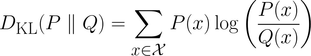
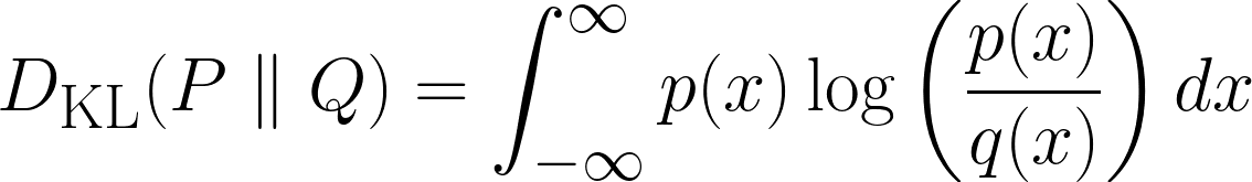
Above is the formula for discrete cases, and the formula below is for continuous cases.

Intuition behind KL-Divergence

In this section, we will intuitively derive the KL-Divergence.  Let’s start off by asking you a series of questions.

Understanding surprise

“If you flipped a coin and I guessed the outcome perfectly, would you be surprised?”. I assume you would be a little surprised but not completely shocked. Now, let's move to the second scenario.

“If you rolled a dice and I guessed the outcome perfectly, would you be more surprised than the previous scenario?”. I assume you would say yes, since it is less probable for me to guess the correct outcome.

Now, one last scenario:

“If I correctly guessed what lottery numbers would win, would you now be more surprised than the previous scenario?”. I assume you would say yes and be in complete shock. But why?

It is because as we progressed through the scenarios, the probability of me being able to guess the correct outcome reduced, and therefore your surprise increased at the outcome. So we have just noticed a relationship:

The probability of an event happening has an inverse relationship to surprise. 

For clarity, as the probability of even happening reduces, the surprise increases, and vice versa. 

However, we can make another interesting observation here. If we go back to the dice rolls, and imagine the scenario where you roll the same dice 3 times, and I guessed it correctly every time, how much more surprised would you be than if there was only 1 dice and I guessed it correctly. 

Well, your surprise wouldn’t be just slightly higher than a single correct guess; it would be dramatically higher, ideally three times higher. Why? Because each new correct guess compounds your disbelief. It’s not just adding a fixed amount of surprise—it’s multiplying how unbelievable the situation feels.

Therefore, when trying to mathematically define Surprise, we would want it to have:

1. Additive property: If two independent events happen, their combined surprise should be the sum of their individual surprises.
1. Example: Guessing 1 die roll correctly → Surprise = S. Guessing 2 die rolls correctly → Surprise = S + S = 2S.
2. Inverse relationship with probability. The less likely an event, the more surprising it is.
1. Example: A coin flip (50%) is less surprising than winning the lottery (0.000001%).
3. Zero surprise for certain events. If something always happens (probability = 1), surprise should be zero.
1. Example: "The sun rose today." → Not surprising at all.
4. Continuous scaling. A small change in probability should lead to a smooth, logical change in surprise (no sudden jumps).

At first glance, since there are a lot of requirements, we would think that the mathematical definition will be quite complicated. However, it is not!

All of the above requirements can be solved by manipulating the logarithm function. The standalone log function (a lot of the time, log(x) and ln(x) are stated interchangeably) has the following shape:

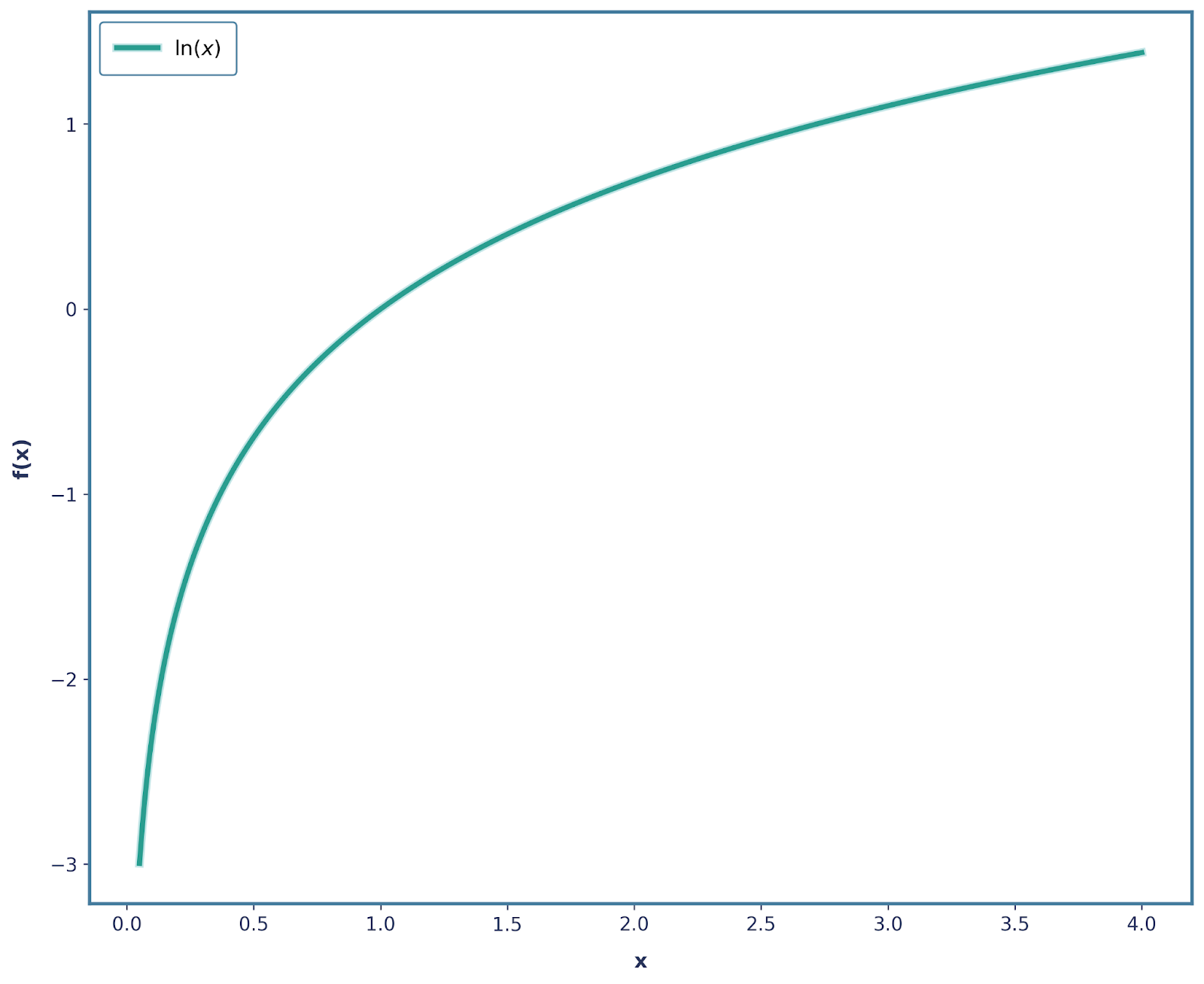
Already we have met quite a lot of our requirements. Let’s focus on the Additive Property first. Remember how we said that if two independent events happen, their total surprise should be the sum of their individual surprises? Well, this is exactly what the log function does!

Here’s how:

The probability of rolling a 6 on a fair die is ⅙ , and let’s define the surprise of the event as this:

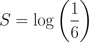
Now, take the event of rolling a 6 three times in a row, the combined probability would be: ⅙ * ⅙ * ⅙ = 1/216. 

In terms of surprise, it would be:

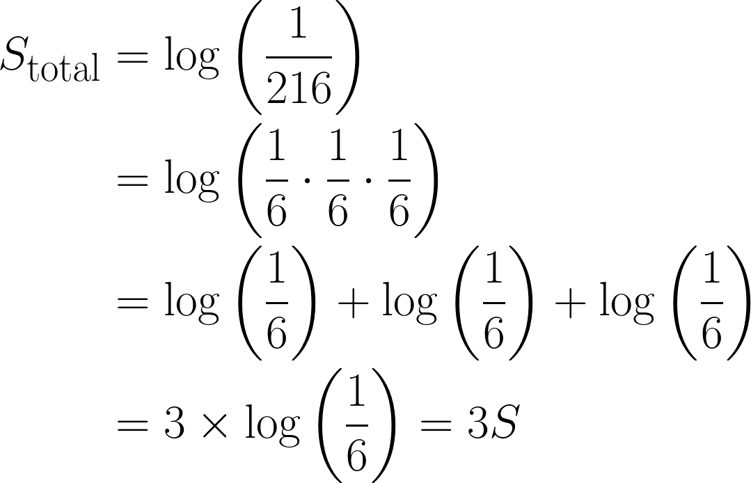
This is quite an important observation, since the total surprise has increased by a factor of 3, due to the logarithm we used. Moreover, this also satisfies Property 3, where log(1) = 0, since an event with full certainty has no element of surprise. 

Additionally, Property 4 is also satisfied as log(x) is a continuous monotonic function! However, Property 2 is not satisfied, as our surprise decreases when the probability decreases (since it becomes more negative). 

We can solve this quite easily, by applying a negative sign! Thus, our function now is -log(x), which has this below shape. 

It is also important to note that all of the other 3 properties are also still satisfied with this change. Therefore, we can mathematically define surprise to  be: 

Entropy

In machine learning, we’re not just interested in the surprise of a single event, but the average surprise across all possible events. That’s called the expected surprise. More specifically, we are interested in finding the expected surprise of the distribution.

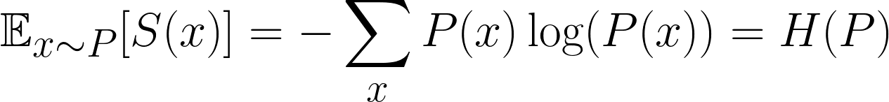
This is a famous formula, and it is the expected surprise, or more commonly known as Entropy. Rather confusingly, however, we often use P and Q to denote our distributions, so don’t get confused with p, which denotes probability!

Intuitively speaking, all we are doing is multiplying the probability of each outcome by its surprise, and then summing across all possible outcomes.

From this point on, we are going to state that P(x) is our true underlying distribution and Q(x)is the distribution we are trying to approximate P(x)with (i.e Q(X)is the “wrong” distribution). This is very common in machine learning—our models are constantly trying to estimate the real world.

So now comes the big question:

What happens if we calculate our surprise using the wrong distribution?

We can still compute surprise, but instead of using P(x), we now measure it with respect to Q(x). This gives us a new expectation:

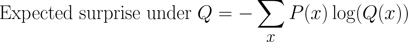
This is often a confusing step when deriving KL-Divergence. We’re still sampling according to P(x) (because that’s what the true distribution is), but we’re measuring surprise using Q(x)(our model’s belief).

This quantity is sometimes called the cross-entropy between P(x)and Q(x).

KL-Divergence Formula

Up until this point, we have defined two quantities:

1. Entropy: the expected surprise if we use the true distribution P(x)
2. Cross-entropy: the expected surprise if we use the wrong distribution Q(x)

To obtain the KL-Divergence formula, we simply subtract these two quantities and obtain this: 

And yes, the question you will have is why? 

Let’s go back to the intuition of surprise.

• Entropy tells us the minimum amount of surprise possible if we knew the true distribution P(x). Think of it as the “ideal cost.”
• Cross-entropy tells us the actual amount of surprise we incur when using the approximation Q(x). Think of it as the “real cost.”

So when we compute the KL-Divergence through subtracting these quantities, we are asking how much extra surprise we are paying because we used the wrong distribution Q(x) instead of the real one P(x). It’s the penalty for having the wrong beliefs.

An important thing to also note is that if Q(x) is the same as P(x), then the KL-Divergence will be equal to 0. This makes sense—if our model's predictions perfectly match the true distribution, then there’s no extra surprise, and hence no penalty.

This is different from cross-entropy, which doesn’t go to zero even when P(x) is equal to Q(x); it just equals the entropy of P(x).

So we can think of KL-Divergence as being "anchored" at zero, meaning it only starts increasing when our predicted distribution begins to diverge from the true one. 

Examples

Great job in deriving the equation! To solidify our concept, let’s do an example to solidify this concept. 

Imagine we are tasked in predicting a user’s favourite movie genre. From past data, we have been given the true distribution over the four movie genres (i.e this is our P(x)). 

Now together, we have built a model which predicted this (i.e this is our Q(x)).

There is clearly some difference in our distribution, but by how much? This is where we will be using the KL-Divergence, using the equation below:

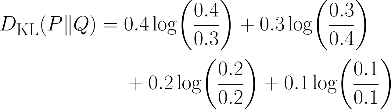
Notice how the term becomes 0 when the two distributions have the same probability for that outcome. 

Coding

We can also solve the above problem using Python:

import numpy as np
from scipy.stats import entropy      # Important module from scipy

P = np.array([0.4, 0.3, 0.2, 0.1])   # This is our true distribution
Q = np.array([0.3, 0.4, 0.2, 0.1])   # This is our model’s prediction

kl_nats = entropy(P, Q)              # natural log ⇒ nats
kl_bits = entropy(P, Q, base=2)      # log₂ ⇒ bits

print(f"KL(P‖Q) = {kl_nats} nats")
print(f"KL(P‖Q) = {kl_bits} bits")

This code is quite simple and intuitive, apart from the fact that we haven’t used the term KL-Divergence in the code anywhere! Rather, I have used entropy many times. 

This brings us to an important point - KL-Divergence is often called Relative Entropy. Therefore, we are in fact calculating the KL-Divergence since the entropy module is calculating the relative entropy between the two distributions. 

This seems to be confusing, so I want to take a brief pause and summarize everything:

Properties of KL-Divergence

Now that we’ve computed our first example using the KL-Divergence formula, let’s take a moment to explore some of its most important properties.

1. Non-negativity: KL-Divergence is never negative. This makes sense intuitively, since the lowest value that it can take is 0, which is when our predicted distribution is exactly equal to the true distribution. And we can never have a negative cost since we cannot be “less surprised” than the theoretical minimum surprise.
2. Anchored at zero: KL-Divergence gives us zero when our predicted distribution matches the true distribution.
3. Units: Bits vs nats: When we calculate KL-Divergence, we use logarithms. But the base of that logarithm determines the unit of the final result:

• If we use log base 2, the result is measured in bits
• If we use natural log (ln), the result is measured in nats (short for “natural units of information”)

4. Asymmetry: This is an important property - KL-Divergence is not symmetric. Using Q(x)to approximate P(x) gives us a different value than using P(x) to approximate Q(x). This is why KL-Divergence isn’t a true distance metric - it doesn’t behave like normal distances.

Applications of KL-Divergence in Machine Learning

KL-Divergence is useful in many different areas in Machine Learning:

• Model evaluation: measuring how far off your predictions are from true labels
• Variational Inference: minimizing DKL, such as in Variational Autoencoders.
• Reinforcement Learning: Trust Region Policy Optimization (TRPO) uses KL constraints
• Language Modeling: comparing token predictions to ground truth

KL-Divergence is closely related to Maximum Likelihood Estimation (MLE), which is a foundational method for estimating model parameters. To learn more about MLE and how it complements the concepts we've covered here, check out my detailed tutorial, Introduction to Maximum Likelihood Estimation (MLE).

Limitations of KL-Divergence and Solutions 

Like all things, there are also limitations in using KL-Divergence. Let’s explore them in detail:

1. Support mismatch blows up KL: In rare cases where Q(x)=0 and P(x)>0, the fractional term log(P/Q) term becomes infinite. To solve this we can add ε‑smoothing or switch to Jensen–Shannon divergence.
2. High‑cardinality categorical features: Having multiple are values would lead to sparse counts and noisy KL estimates. To fix this, we can merge rare categories or apply Bayesian smoothing.
3. Asymmetry can be quite misleading: This is because KL(P || Q) and KL(Q || P) do not produce the same value. A potential fix is using Jensen-Shannon Divergence
4. Units: A lot of times, we tend to forget to include the units of KL-Divergence, and this becomes especially problematic since both nats and bits are commonly used. So always state the log base!

Jensen-shannon divergence

You might have noticed I included Jensen-Shannon Divergence before, so let’s quickly go through it. 

Although it is slightly more complicated and computationally heavier than KL-Divergence, Jensen-Shannon Divergence is symmetric. It still is not a true distance metric since it doesn’t satisfy the triangular inequality. However, if we square root the JS-Divergence, then it does satisfy the triangle inequality and becomes a proper metric. 

It is also a smoothed version of KL‑divergence that always stays between 0 and 1 bit (if we use log base 2). If we look at the equation again, each KL term is measured against the shared midpoint M, neither P nor Q will ever divide by zero, and therefore, no infinities.

Conclusion

In short, KL‑Divergence is an important tool that we use to measure the extra information cost we have when we let our model’s distribution Q stand in for the true distribution P. It becomes zero if they are the same, and larger when they aren’t, and always non‑negative. KL-Divergence connects entropy and cross‑entropy, and it shows up in loss functions, variational inference, and policy constraints. 

Now KL-Divergence is great but it is still a tool we use when dealing with Machine Learning and Deep Learning related problems. To be able to apply this further be sure to check out our Machine Learning Scientist in Python career track and our Machine Learning Engineer career track, where both explore supervised, unsupervised, and deep learning. 

If you are also ready to start linking KL-Divergence with further Mathematical concepts, then check out these resources:

• Cross-Entropy Loss Function in Machine Learning: Enhancing Model Accuracy: Learn how cross-entropy is used to optimize model accuracy in both Pytorch and Tensorflow.
• Demystifying Mathematical Concepts for Deep Learning: Explore full coverage of important Mathematical concepts in Deep Learning, along with code in Python.
• Understanding Data Drift and Model Drift: Drift Detection in Python: Explore how KL-Divergence can be used to solve an important problem in ML - Model Drift.