Python Polars Tutorial: A Complete Guide for Beginners

In the world of data analysis, pandas has long been the default choice for handling tabular data in Python by data professionals. 

However, as datasets grow in size and complexity, pandas can encounter performance bottlenecks, limited multi-core utilization, and memory constraints.

This is where Polars emerges as a modern alternative. Polars is a DataFrame library written in Rust that provides blazing-fast performance, efficient memory management, and a design philosophy focused on scalability.

In this tutorial, we’ll share what Polars is and how to perform some basic Polars operations in Python. If you're looking for some hands-on experience, I recommend checking out the Introduction to Polars course.

Key Features of Python Polars

Polars offers a unique set of features that set it apart from pandas:

• Rust foundation: Safety and performance at the systems level.
• Multi-threaded execution: Makes full use of modern CPUs.
• Lazy evaluation: Defers execution until explicitly required.
• Schema enforcement: Ensures consistent data handling.
• Advanced data type support: Handles temporal, categorical, and nested types natively.

Data types in Polars

Polars supports a wide range of data types beyond the basics:

• Numeric: Int32, Int64, Float32, Float64.
• Boolean: true/false values.
• Temporal: Date, Datetime, Duration, Time.
• Categorical: Encoded strings for memory-efficient storage.
• Nested: List and Struct types, useful for JSON-like data.

Advantages Over pandas

Being the newer and more modern alternative to pandas, Polars offers several benefits:

• Faster execution on large datasets.
• More memory-efficient.
• Better suited for ETL pipelines and production.
• Built-in optimizations like predicate and projection pushdown.

Installation and Environment Setup for Python Polars

Now, let’s have a look at how we can start using Polars for ourselves in Python.

Before using Polars, you need to set up the environment correctly.

Supported Platforms

Polars supports Windows, macOS, and Linux. It can be installed in virtual environments, system Python, or via containerized workflows (Docker).

Installation with pip

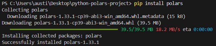
To install the polars library in Python, run the following command in terminal.

pip install polars

You should see the following installation message:

Installation with conda

Alternatively, you can install the library in the conda environment if that’s what you’re working with.

conda install -c conda-forge polars

Verify Installation

To check if your installation has run successfully, write the following simple script:

import polars as pl
print(pl.__version__)

Configuration and Environment Variables

Polars lets you tune how it runs and how its outputs are displayed by setting environment variables before starting your Python session. For example:

• POLARS_MAX_THREADS: Limit the number of threads.
• POLARS_FMT_MAX_COLS: Control the number of columns printed.
• POLARS_FMT_TABLE_WIDTH: Adjust DataFrame display width.

Here’s an example of how you would set these variables in a shell before running Python:

export POLARS_MAX_THREADS=8
export POLARS_FMT_MAX_COLS=20

Generating a Sample CSV Dataset for Demonstration

Before diving into the features of Polars, it’s helpful to have a dataset that we can use consistently throughout this tutorial. We can generate a simple CSV file using Python’s built-in csv module or pandas. 

Here is an example that creates a transactions.csv file with synthetic data:

import csv
import random
from datetime import datetime, timedelta

# Define column names
columns = ["transaction_id", "customer_id", "amount", "transaction_date"]

# Generate synthetic rows
rows = []
start_date = datetime(2023, 1, 1)
for i in range(1, 101):
    customer_id = random.randint(1, 10)
    amount = round(random.uniform(10, 2000), 2)
    date = start_date + timedelta(days=random.randint(0, 90))
    rows.append([i, customer_id, amount, date.strftime("%Y-%m-%d")])

# Write to CSV
with open("transactions.csv", "w", newline="") as f:
    writer = csv.writer(f)
    writer.writerow(columns)
    writer.writerows(rows)

This script creates a dataset of 100 transactions with random amounts, customer IDs, and transaction dates. You can adjust the range and size to suit your needs. 

Save this script, run it once, and you’ll have a CSV file to use in the examples throughout this article.

Core Concepts in Python Polars DataFrames and Series

Polars is built on a foundation of two core abstractions: the Series and the DataFrame. 

Together, they provide a structured, efficient way of working with data, similar in spirit to pandas, but optimized with Polars’ Rust-powered backend. Let’s break down the main concepts.

Series: 1D arrays with a defined type

A Series in Polars is a one-dimensional array, similar to a column in a spreadsheet or database table. Each Series has:

• A name (the column label).
• A data type (such as Int64, Utf8, Float64, Boolean, etc.).
• An ordered collection of values.

Because the data type is strictly enforced, Series in Polars tend to be faster and more predictable than Python lists.

Example:

import polars as pl
# Create a Series of integers
s = pl.Series("numbers", [1, 2, 3, 4, 5])
print(s)

Output:

shape: (5,)
Series: 'numbers' [i64]
[
    1
    2
    3
    4
    5
]

DataFrame: A collection of series

A DataFrame is a two-dimensional structure that organizes multiple Series together under a schema. Conceptually, it’s like a table in SQL or Excel. Rows represent records, and columns represent fields.

Example:

df = pl.DataFrame({
    "id": [1, 2, 3],
    "name": ["Alice", "Bob", "Charlie"],
    "age": [25, 30, 35]
})
print(df)

Output:

shape: (3, 3)
┌─────┬─────────┬─────┐
│ id  │ name    │ age │
│ --- │ ---     │ --- │
│ i64 │ str     │ i64 │
├─────┼─────────┼─────┤
│ 1   │ Alice   │ 25  │
│ 2   │ Bob     │ 30  │
│ 3   │ Charlie │ 35  │
└─────┴─────────┴─────┘

Each column is a Series, and the DataFrame enforces its schema.

Role of schemas and strict type consistency

One of Polars’ strengths is strict schema enforcement. Each column has a fixed data type, and Polars ensures all operations respect it. This prevents subtle bugs that arise in dynamically typed operations.

For instance, you cannot accidentally add a string column to an integer column without explicit conversion.

Example:

df = df.with_columns(
    (pl.col("age") + 5).alias("age_plus_5")
)
print(df)

Here, age is i64, and the result remains an integer. If you tried adding a string column, Polars would raise an error instead of silently failing.

Null Handling

Real-world data often has missing values, and Polars provides clear tools for dealing with them:

• fill_null(): Replace nulls with a given value.
• drop_nulls(): Remove rows containing nulls.
• is_null() / is_not_null(): Boolean checks.

Expressions: Vectorized Column Operations

Polars promotes an expression system, where operations are defined as transformations on columns rather than row-by-row Python loops. 

These expressions are vectorized, meaning they operate on entire columns at once, which is much faster.

Instead of manually looping, Polars builds a fast vectorized computation.

Eager vs. Lazy Execution

Polars offers two modes of execution:

1. Eager Execution

• Runs computations immediately.
• Similar to pandas.
• Great for interactive exploration and small-to-medium datasets.

Here’s an example of an eager execution:

df = pl.DataFrame({"x": [1, 2, 3]})
print(df.select(pl.col("x") * 2))  # eager: runs instantly

2. Lazy Execution

• Builds a query plan instead of executing right away.
• Polars optimizes this plan under the hood (predicate pushdown, parallelization, projection pruning).
• Ideal for large datasets and complex transformations.

Here’s an example of a lazy execution:

lazy_df = pl.DataFrame({"x": [1, 2, 3]}).lazy()
result = lazy_df.select(pl.col("x") * 2).collect()  # execute on collect()
print(result)

Here, nothing is computed until .collect() is called. In large workflows, this can lead to dramatic performance improvements.

Basic DataFrame Operations in Python Polars

Next, we’ll look at performing some basic operations used in Polars on the dataset we created.

Loading the dataset

Polars can ingest data from multiple file formats and memory objects. This makes it flexible for integrating into modern data pipelines.

Here's how you can do that for different sources:

From CSV dataset we created earlier:

import polars as pl

df = pl.read_csv("transactions.csv")
print(df.head())

We can also read the dataset in from Parquet if required.

df_parquet = pl.read_parquet("transactions.parquet")

If you have a JSON file instead, you can read it using this code:

df_json = pl.read_json("transactions.json")
#For JSON Lines (NDJSON), use the following instead:
df_json = pl.read_ndjson("transactions.json")

Here’s how you read datasets from an Arrow Table:

import pyarrow as pa

arrow_table = pa.table({
    "transaction_id": [1, 2],
    "customer_id": [5, 7],
    "amount": [150.25, 300.75],
    "transaction_date": ["2023-01-02", "2023-01-03"]
})
df_arrow = pl.from_arrow(arrow_table)

Selecting and Filtering

Now let’s pick specific columns or rows from our dataset.

Select Columns

When using Polars, a common operation is to select the columns you want to work on and keep. 

Here’s how you can do that:

# Select only transaction_id and amount
df.select(["transaction_id", "amount"])

Filter Rows

You can also filter rows based on conditions you set, similar to pandas.

# Get only high-value transactions above $1,000
high_value = df.filter(pl.col("amount") > 1000)
print(high_value)

Apply Expressions

Applying expressions in Polars involves using the polars.Expr object within various contexts to perform data transformations.

You can create them using pl.col(), or pl.lit().

# Add a 10% discount column to simulate promotional pricing
df.select([
    pl.col("transaction_id"),
    pl.col("amount"),
    (pl.col("amount") * 0.9).alias("discounted_amount")
])

Aggregations

We can analyze spending patterns by customer using group_by.

# Total and average spend per customer
agg_df = df.group_by("customer_id").agg([
    pl.sum("amount").alias("total_spent"),
    pl.mean("amount").alias("avg_transaction")
])
print(agg_df)

Sample output:

shape: (10, 3)
┌─────────────┬────────────┬───────────────┐
│ customer_id │ total_spent│ avg_transaction│
│ ---         │ ---        │ ---           │
│ i64         │ f64        │ f64           │
├─────────────┼────────────┼───────────────┤
│ 1           │ 5230.12    │ 523.01        │
│ 2           │ 6120.45    │ 680.05        │
│ ...         │ ...        │ ...           │
└─────────────┴────────────┴───────────────┘

Handling Missing Values

Our generated dataset has no nulls by default, but let’s simulate how we’d handle them.

Fill Missing Values

Missing values can cause issues in downstream analysis and data visualization. You’ll need to fill in any missing values to ensure things are smooth.

Here’s how you can fill missing values:

# Imagine 'amount' has missing values, then replace with 0
df_filled = df.with_columns(
    pl.col("amount").fill_null(0)
)

Drop Nulls

Nulls can cause errors if not dealt with. Here’s how to drop them:

df_no_nulls = df.drop_nulls()

Convert Types

Data types might be incorrectly formatted in a dataset. Here’s how you can convert them using the .cast method:

# Ensure customer_id is treated as string instead of int
df_casted = df.with_columns(
    pl.col("customer_id").cast(pl.Utf8)
)

Chaining Operations

Polars allows method chaining for cleaner workflows. This chaining method is commonly used in SQL or R programming using the tidyverse package.

Example: Find top customers in March by total spend

pipeline = (
    df
   .with_columns(pl.col("transaction_date").str.strptime(pl.Date, format="%Y-%m-%d"))
    #.col("date_str").str.to_date(format="%Y-%m-%d")
    .filter(pl.col("transaction_date").dt.month() == 3)  # transactions in March
    .group_by("customer_id")
    .agg(pl.sum("amount").alias("march_spent"))
    .sort("march_spent", descending=True)
)
print(pipeline)

This pipeline:

1. Filters March transactions.
2. Groups by customer.
3. Aggregates spending.
4. Sorts by total spend.

This chaining method allows a pipeline analysis to be done without using intermediate DataFrames.

Advanced Features and Lazy Evaluation in Polars

Beyond the basics, Polars shines when working with large datasets thanks to its lazy evaluation engine. This model allows Polars to build a query plan first, optimize it under the hood, and only then execute the pipeline. The result is a huge boost in performance and efficiency, especially with millions of rows or complex transformations.

By default, Polars runs in eager mode. This means computations happen immediately, similar to pandas. Lazy mode, however, works differently:

• Each operation (filter, select, group_by) is recorded instead of executed right away.
• The transformations are only executed when you call .collect().
• This defers work until Polars can analyze the whole pipeline and run it in the most efficient way possible.

Here’s a lazy mode example:

import polars as pl

# Load dataset in lazy mode
lazy_df = pl.scan_csv("transactions.csv")

# Build a transformation pipeline
pipeline = (
    lazy_df
    .filter(pl.col("amount") > 1000)                # step 1: filter expensive transactions
    .group_by("customer_id")                         # step 2: group by customer
    .agg(pl.sum("amount").alias("total_spent"))     # step 3: aggregate
)

# Nothing has run yet, computation happens only on collect()
result = pipeline.collect()
print(result)

Query Optimization

Polars optimizes queries by applying pushdown techniques:

1. Predicate Pushdown: Filters are pushed as close to the data source as possible. Example: When filtering amount > 1000, Polars applies that filter while reading the CSV instead of after loading all rows.
2. Projection Pushdown: Only the columns you need are read into memory. Example: If you only select customer_id and amount, Polars skips reading transaction_date entirely.

Streaming for Large Data

When data is too large to fit into memory, Polars offers streaming execution. Instead of loading everything at once, Polars processes data in batches, keeping memory usage stable.

This is especially useful for multi-GB CSV or Parquet files.

Example (streaming mode):

# Enable streaming execution for huge datasets
stream_result = (
    lazy_df
    .group_by("customer_id")
    .agg(pl.sum("amount").alias("total_spent"))
    .collect(streaming=True)   # execute in streaming mode
)

With streaming=True, Polars avoids building massive in-memory intermediate tables, making it more scalable than pandas for large workloads.

Execution with .collect() and Debugging Lazy Queries

The .collect() method is the trigger for executing a lazy pipeline. Before that, you can inspect and debug the query plan with:

• .describe_plan(): Shows the logical plan.
• .describe_optimized_plan(): Shows the optimized plan after Polars applies pushdowns and simplifications.

Optimizing Python Polars Performance and Efficiency

Polars can help boost performance in running your analysis pipelines.

Here are some best practices:

• Use lazy evaluation for large pipelines.
• Minimize type casting.
• Avoid unnecessary materialization of intermediate DataFrames.

Joins, Merging, and Combining Data in Python Polars

Real-world analysis often requires combining datasets. Polars provides a full suite of join operations with optimized execution, making it easy to merge even large tables.

Supported Joins

Polars supports all major join types:

• Inner Join: Keep only matching rows.
• Left / Right Join: Keep all rows from one side.
• Outer Join: Keep all rows, filling missing with nulls.
• Semi Join: Keep left rows that have a match on the right.
• Anti Join: Keep left rows that don’t have a match on the right.
• Cross Join: Cartesian product of both tables.

Example: Joining transactions with customer metadata

# Create customer metadata DataFrame
customers = pl.DataFrame({
    "customer_id": [1, 2, 3, 4, 5],
    "customer_name": ["Alice", "Bob", "Charlie", "David", "Eva"]
})

# Inner join on customer_id
df_joined = df.join(customers, on="customer_id", how="inner")
print(df_joined.head())

Polars vs Pandas joins for performance and usability

Polars is superior to Pandas in both areas:

• Performance: Polars joins are implemented in Rust with parallelism, making them faster on large datasets than pandas. Predicate and projection pushdown also apply to joins, reducing unnecessary data movement.
• Usability: Polars requires explicit join keys, which avoids accidental joins on index alignment (a common pitfall in pandas). Semi and anti joins are native in Polars, while in pandas they require workarounds.

Window Functions and Rolling Operations in Polars

Window functions allow calculations within groups or over ordered rows, without collapsing results, similar to SQL window functions.

Polars lets you compute statistics per customer or per time period using window contexts.

Here are some examples of window functions you can use in Polars:

• Rolling mean/sum for moving averages.
• Expanding windows for cumulative stats.
• Ranking functions for order-based analytics.

1. Running functions

Example: Customer running totals

df_window = df.with_columns( pl.col("amount") .sort_by("transaction_date") .cum_sum() .over("customer_id") .alias("running_total") )
print(df_window.head())

2. Rolling functions

Rolling functions operate over a sliding window of rows or time.

Example: 7-day rolling sum of transactions

df = df.with_columns(pl.col("transaction_date").str.strptime(pl.Date, format="%Y-%m-%d")
rolling = (
    df.group_by_rolling("transaction_date", period="7d")
      .agg(pl.sum("amount").alias("rolling_7d_sum"))
)
print(rolling.head())

Expanding windows (cumulative) and center-aligned windows are also supported by adjusting parameters.

3. Ranking functions

You can use ranking functions and custom aggregations inside windows.

Example: Rank transactions per customer by amount

ranked = df.with_columns(
    pl.col("amount").rank("dense", descending=True).over("customer_id").alias("rank")
)
print(ranked.head())

This produces rankings (1 = highest) for each customer’s spending.

Window functions allow contextual calculations:

print(
    df.group_by("customer_id").agg(pl.col("amount").cum_sum().alias("cumulative_spent"))
)

Using SQL Queries in Python Polars

For analysts used to SQL, Polars provides a SQL context so you can query DataFrames directly with SQL syntax while still leveraging Polars’ speed.

SQL Context and DataFrame Registration

To start, you must register a DataFrame before running SQL.

from polars import SQLContext

ctx = SQLContext()
ctx.register("transactions", df)

Running SQL Queries Directly in Polars

Let’s look at an example of how to run a SQL query within Python using Polars.

Example: Query total spend per customer in SQL

result = ctx.execute("""
    SELECT customer_id, SUM(amount) AS total_spent
    FROM transactions
    GROUP BY customer_id
    ORDER BY total_spent DESC
""").collect()

print(result)

Integrating SQL with Polars Expressions

You can mix SQL and expressions:

sql_result = ctx.execute("SELECT * FROM transactions WHERE amount > 1500")
df_sql = sql_result.collect()

# Continue with Polars expressions
df_sql = df_sql.with_columns((pl.col("amount") * 0.95).alias("discounted"))

This is useful for teams transitioning from SQL-based tools.

Integration of Python Polars with the Wider Ecosystem

Polars is designed not as a standalone island, but as a high-performance DataFrame library that plays well with the broader Python data ecosystem. This interoperability ensures analysts and engineers can adopt Polars incrementally while still leveraging existing tools.

Here are some areas of integration:

• Package interoperability: Seamlessly convert between Polars, pandas, NumPy, Arrow.
• Visualization: Use matplotlib, seaborn, or plotly for charting.
• Machine learning: Feed Polars DataFrames into scikit-learn, PyTorch, or TensorFlow pipelines.
• Cloud & DB: Efficient I/O with Parquet, Arrow, and connectors for cloud storage.
• Jupyter notebooks: Polars integrates smoothly into interactive environments.

Python Polars Examples and Common Use Cases

Lastly, let’s have quick look at some examples of Polars being used:

1. Data cleaning

df = df.with_columns([
    pl.col("transaction_date").str.strptime(pl.Date, "%Y-%m-%d").alias("txn_date"),
    pl.col("amount").fill_null(strategy="mean")
])

2. ETL pipelines

result = (
    pl.read_csv("transactions.csv")
      .lazy()
      .filter(pl.col("amount") > 1000)
      .group_by("customer_id")
      .agg(pl.sum("amount").alias("total_spent"))
      .collect()
)

3. Finance

Here’s an example for rolling averages for transaction amounts.

import polars as pl

# Load & parse dates
df = (
    pl.read_csv("transactions.csv")
    .with_columns(pl.col("transaction_date").str.strptime(pl.Date, "%Y-%m-%d"))
)

# (A) Overall: daily totals + 7-day rolling average
daily = (
    df.sort("transaction_date")
      .group_by_dynamic("transaction_date", every="1d")
      .agg(pl.sum("amount").alias("daily_total"))
      .sort("transaction_date")
      .with_columns(
          pl.col("daily_total").rolling_mean(window_size=7).alias("ma7")
      )
)

# (B) Per-customer: daily totals + 7-day rolling average within each customer
daily_by_cust = (
    df.sort("transaction_date")
     .group_by_dynamic(index_column="transaction_date", every="1d", by="customer_id")
      .agg(pl.sum("amount").alias("daily_total"))
      .sort(["customer_id", "transaction_date"])
      .with_columns(
          pl.col("daily_total")
            .rolling_mean(window_size=7)
            .over("customer_id")
            .alias("ma7_per_customer")
      )
)

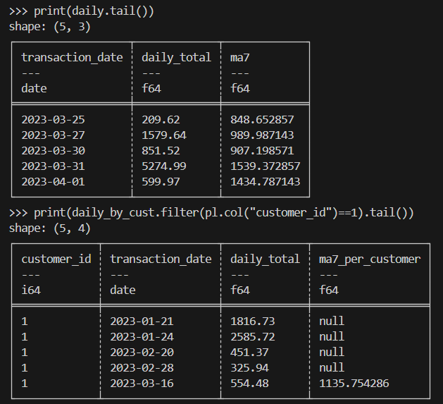
print(daily.tail())
print(daily_by_cust.filter(pl.col("customer_id")==1).tail())

Here’s the expected result:

4. Scientific computing

When doing scientific computing, you’ll need to handle millions of rows of experimental or simulated transaction-like data efficiently.

Here’s a sample implementation:

import polars as pl

# Assume a very large Parquet file with columns: id, value, ts (UTC)
# Use lazy scan_* to avoid loading into memory up-front
lazy = (
    pl.scan_parquet("experiments.parquet")           # or: pl.scan_csv("experiments.csv")
      .filter(pl.col("value") > 0)                   # predicate pushdown
      .select(["id", "value", "ts"])                 # projection pushdown
      .with_columns(
          # Example transformations: standardization & bucketize timestamps by hour
          ((pl.col("value") - pl.col("value").mean()) / pl.col("value").std())
              .alias("z_value"),
          pl.col("ts").dt.truncate("1h").alias("ts_hour")
      )
      .group_by(["id", "ts_hour"])
      .agg([
          pl.len().alias("n"),
          pl.mean("z_value").alias("z_mean"),
          pl.std("z_value").alias("z_std")
      ])
      .sort(["id", "ts_hour"])
)

# Execute in streaming mode to keep memory usage low
result = lazy.collect(streaming=True)

# Optionally write out partitioned Parquet for downstream analysis
result.write_parquet("experiments_hourly_stats.parquet")
print(result.head())

Final Thoughts

Python Polars provides a modern, high-performance DataFrame library that addresses many of pandas’ limitations. While pandas remains popular for smaller, ad-hoc analysis, Polars is increasingly the tool of choice for scalable, efficient, and reliable data processing in Python.

Want to learn more about Polars? You will love our Introduction to Polars course or our Introduction to Polars article. Our Polars Engine article might interest you as well.