SUMPRODUCT() Excel: What You Should Know

Before functions like SUMIF() and SUMIFS() existed, SUMPRODUCT() was one of Excel’s primary tools for handling conditional logic. Analysts used it to filter data, apply multiple criteria, and calculate weighted results long before dedicated conditional functions were introduced.

Even today, SUMPRODUCT() handles scenarios that newer functions struggle with, especially when multiple conditions, arrays, or calculations need to be evaluated together.

Despite this, it is either overlooked or misunderstood. Many users know it exists, but never move beyond basic examples. 

In this article, you’ll learn how to use SUMPRODUCT() for conditional and weighted calculations, and how to avoid common errors so you can use it confidently in real-world Excel models.

Understanding SUMPRODUCT()

SUMPRODUCT() is an Excel function that multiplies corresponding values in arrays and then sums the results, so you can perform complex calculations in a single formula. While it’s frequently associated with advanced analysis, its original purpose was far more practical.

Fundamental concepts and basic syntax

The SUMPRODUCT() function in Excel takes two or more ranges, multiplies their corresponding values, and sums the results into a single final value. Its core purpose is to combine calculation and aggregation into a single formula and eliminate the need for additional helper columns.

This means that no matter how many arrays you include, SUMPRODUCT() always produces one numeric result.

The syntax of SUMPRODUCT() is:

SUMPRODUCT(array1, [array2], …)

Here’s a breakdown of this syntax: 

When you use SUMPRODUCT(), consider the following: 

• Each array must have the same number of rows and columns because SUMPRODUCT() aligns items by position. 

• If one array is longer or shaped differently, the function can’t match the values correctly and may throw a #VALUE! error.

• Blank cells are treated as zeros.

• Text is ignored in calculations unless used in a logical expression. 

Default behavior: Multiplication and summation

By default, SUMPRODUCT() multiplies corresponding values from multiple arrays and then adds the results together. This element-by-element multiplication followed by summation is how the function works. 

For example, if we have a simple dataset with quantities and prices. If the Quantity column contains quantities and the Price column contains prices, the following formula calculates total revenue:

=SUMPRODUCT(A2:A4, B2:B4)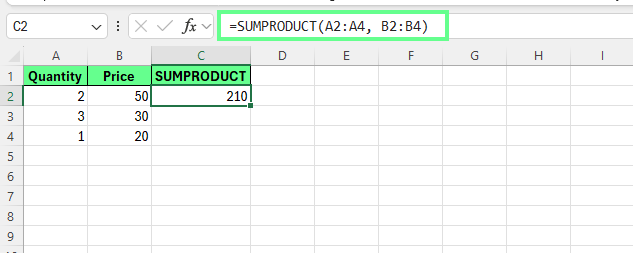

SUMPRODUCT() in Excel. Image by Author.

Behind the result, Excel evaluates each row individually and then sums the results:

• Row 1: 2 × 50 = 100
• Row 2: 3 × 30 = 90
• Row 3: 1 × 20 = 20

Excel then adds those values together: 100 + 90 + 20 = 210

This replaces the need for helper columns that manually calculate row-level totals before summing them. SUMPRODUCT() keeps the entire calculation in a single formula to reduce formula sprawl and lowers the risk of referencing errors.

This default multiply-then-sum behavior enables more advanced uses later, including conditional logic and weighted calculations.

Extending SUMPRODUCT() Beyond the Basics

Now that you know how it works, let's see some advanced operations SUMPRODUCT() can do:

Advanced arithmetic and operator usage

SUMPRODUCT() can evaluate full arithmetic expressions, including addition, subtraction, and division on a row-by-row basis before summing the results.

When you use arithmetic operators (*, +, -, /) inside an expression, Excel evaluates the entire calculation for each row first. For example, this formula calculates the total revenue minus discounts: 

=SUMPRODUCT((B2:B6*C2:C6)-E2:E6)

This multiplies Quantity × Price for each row and subtracts the Discount value, and then adds all resulting values into a single total.

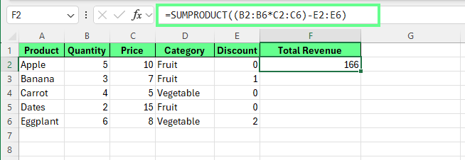
Use arithmetic expressions and operators in SUMPRODUCT(). Image by Author.

However, commas work differently. When you separate arrays with commas, each array is treated as an independent input, and SUMPRODUCT() multiplies corresponding elements across those arrays before summing them. 

To use logical conditions, SUMPRODUCT() relies on the double unary operator --. Logical expressions such as A2:A6>100 return TRUE or FALSE values, which must be converted into 1s and 0s before they can participate in arithmetic. 

The double unary performs that conversion:

=SUMPRODUCT(--(A2:A6>100), B2:B6)

In this example, only rows where the condition is TRUE contribute to the total.

This operator flexibility: combining arithmetic expressions, logical tests, and array pairing is what makes SUMPRODUCT() invaluable for modeling, reporting, and scenarios where helper columns would otherwise be required.

Conditional calculations and logical criteria

SUMPRODUCT() can evaluate logical conditions directly inside a formula. These conditions generate arrays of TRUE and FALSE values, which must be converted into numbers before they can participate in calculations.

Let's say we want to sum the Quantity for products in the Fruit category. In this case, if you try this formula =SUMPRODUCT((D2:D6="Fruit"), B2:B6),  the result is 0. 

Why? That’s because a logical test like this: D2:D6="Fruit" produces {TRUE, TRUE, FALSE, TRUE, FALSE}.

These are logical values, not numbers. And because SUMPRODUCT() performs numeric math, those logical values must be converted into 1s and 0s. The double unary operator -- performs that conversion:

--(D2:D6="Fruit")

This converts logical values into numbers like this:

{1, 1, 0, 1, 0}

Here, TRUE becomes 1 and FALSE becomes 0. Now SUMPRODUCT() can multiply correctly.

=SUMPRODUCT(--(D2:D6="Fruit"), B2:B6)

This is how it calculates: 

(1×5) + (1×3) + (0×4) + (1×2) + (0×6) = 10

Only rows marked with 1 are included in the calculation. The result is 10, which is the total quantity for Fruit products.

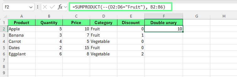
Use Double unary in SUMPRODUCT() in Excel. Image by Author.

Handling multiple criteria (AND/OR Logic)

SUMPRODUCT() handles multiple conditions using AND and OR logic. Let’s see how: 

AND logic: all conditions must be met

To apply AND logic, conditions are multiplied using *. Because only 1 × 1 equals 1, a row is included only when every condition evaluates to TRUE:

=SUMPRODUCT(--(A2:A10>50)* --(B2:B10<100)* C2:C10)

You can also separate arrays with commas. By default, SUMPRODUCT() multiplies comma-separated arrays. But * makes the AND logic easier to see.

=SUMPRODUCT(--(A2:A10>50), --(B2:B10<100), C2:C10)

In this example, values from column C are summed only when:

• Column A is greater than 50
• Column B is less than 100

If either condition fails, the row evaluates to 0 and is excluded.

OR logic: any condition can be met

OR logic is created by adding conditions together using +. If any condition evaluates to TRUE, the row contributes to the total:

=SUMPRODUCT(--((A2:A10>50)+(B2:B10<100)), C2:C10)

Here, rows are included when either condition is TRUE. The addition may produce values greater than 1, but the double unary -- converts any nonzero result into 1, ensuring each row is counted once.

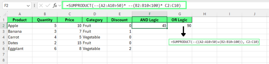
Apply AND and OR logic using SUMPRODUCT(). Image by Author.

Why SUMPRODUCT() is often preferred over SUMIFS()

While SUMIFS() handles multiple AND conditions well, it cannot natively evaluate OR logic or more complex patterns when conditions span multiple columns or mix numeric and text criteria.

SUMPRODUCT() excels in scenarios such as:

• Applying OR logic across columns
• Combining numeric thresholds with text conditions
• Building multi-column filters without helper columns

This flexibility makes SUMPRODUCT() a reliable choice for advanced filtering, modeling, and reporting scenarios where conditional logic goes beyond standard SUMIFS() rules.

Applied Analytical Techniques with SUMPRODUCT()

SUMPRODUCT() is not just for simple calculations; it can handle complex analysis too. 

Row and column criteria applications

SUMPRODUCT() can apply conditions across both rows and columns at the same time. So it’s easier to work with matrix-style or cross-tabulated data. 

Instead of returning a single value like INDEX/MATCH, it can evaluate multiple intersections at once and return a combined total.

This allows SUMPRODUCT() to act as a dynamic two-way lookup without helper columns or separate lookup formulas.

Suppose you have a sales matrix by product (rows) and region (columns), and you want to calculate total sales for Apple and Banana in the North and East regions. 

For this, you’ll use the following formula:

=SUMPRODUCT(
B2:E4 *
  ((A2:A4="Apple")+(A2:A4="Banana")) *
  ((B1:E1="North")+(B1:E1="East"))
)

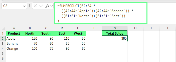
SUMPRODUCT() handles matrix multiplication. Image by Author.

In this formula:

• B2:E4 contains the sales values

• (A2:A4="Apple") + (A2:A4="Banana") creates a vertical row filter

• (B1:E1="North") + (B1:E1="East") creates a horizontal column filter

Rows and columns that meet the criteria evaluate to 1. All others evaluate to 0. Each value in the sales matrix is multiplied by both its row and column conditions.

Only cells that meet both conditions remain non-zero.

In this example:

• Apple (North + East): 120 + 110
• Banana (North + East): 70 + 85

Total: 385

This pattern works for any two-dimensional dataset where multiple row and column conditions need to be applied at once, such as:

• Product × region
• Year × category
• Department × cost type

In these scenarios, SUMPRODUCT() provides more flexibility than traditional lookup functions and avoids the complexity of nested formulas.

Weighted average calculations

Weighted averages are a natural fit for SUMPRODUCT() because the calculation itself follows the function’s default behavior: multiply values by weights, then sum the results.

The standard weighted average formula looks like this:

(Sum of Score × Weight) ÷ (Sum of Weights)

But SUMPRODUCT() simplifies this by handling the multiplication and summation in one step. Instead of creating helper columns, you can calculate the weighted total directly and divide by the sum of the weights:

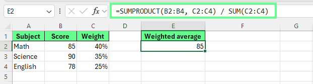
=SUMPRODUCT(values, weights) / SUM(weights)

For example, to calculate a student’s weighted course average, you can use the following formula:

=SUMPRODUCT(B2:B4, C2:C4) / SUM(C2:C4)

Here’s how Excel evaluates each component:

• Math: 85 × 0.40 = 34
• Science: 90 × 0.35 = 31.5
• English: 78 × 0.25 = 19.5

The weighted total is 85, which becomes the final average.

Calculating the weighted average using the SUMPRODUCT. Image by Author.

Filtering or adjusting weights with criteria

Where SUMPRODUCT() becomes more helpful is when weights need to be adjusted dynamically. 

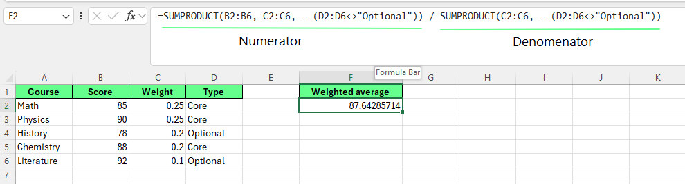
For example, you can exclude certain courses or apply conditions to the calculation:

=SUMPRODUCT(B2:B6, C2:C6, --(D2:D6<>"Optional")) / 
 SUMPRODUCT(C2:C6, --(D2:D6<>"Optional"))

The formula divides the weighted total (numerator) by the total weight (denominator).

Calculating the weighted average using SUMPRODUCT. Image by Author.

In this formula:

• (D2:D6<>"Optional") returns {TRUE, TRUE, FALSE, TRUE, FALSE}

• --(D2:D6<>"Optional") converts to {1, 1, 0, 1, 0}

• Numerator: (85×0.25×1) + (90×0.25×1) + (78×0.20×0) + (88×0.20×1) + (92×0.10×0) = 21.25 + 22.50 + 0 + 17.60 + 0 = 61.35

• Denominator: (0.25×1) + (0.25×1) + (0.20×0) + (0.20×1) + (0.10×0) = 0.70

In this pattern, only rows that meet the condition contribute to both the weighted total and the total weight. This keeps the calculation accurate without restructuring the data or adding helper columns.

Because weighted averages rely on row-by-row multiplication before summation, SUMPRODUCT() is often the most direct and flexible tool for grading models, portfolio weighting, and performance scoring.

Advanced applications and complex scenarios

One of SUMPRODUCT()’s biggest strengths is how easily it combines with other Excel functions. Because it evaluates calculations row by row, it can turn text functions, lookup results, and logical tests into numeric inputs for flexible analysis.

Let’s see how. 

Partial text matches using SEARCH() with SUMPRODUCT()

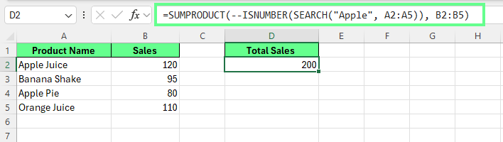
To match text that contains a word or phrase, pair SUMPRODUCT() with SEARCH() and ISNUMBER():

=SUMPRODUCT(--ISNUMBER(SEARCH("Apple", A2:A5)), B2:B5)

In this formula: 

• SEARCH() returns a number when a match is found

• ISNUMBER() converts matches into TRUE/FALSE

• -- converts those values into 1s and 0s

Only rows containing “Apple” contribute to the total.

Combining SUMPRODUCT() with SEARCH(). Image by Author.

Case-sensitive matching using EXACT() with SUMPRODUCT()

By default, Excel text comparisons are not case-sensitive. When case matters, you can use EXACT() inside SUMPRODUCT() like this:

=SUMPRODUCT(--EXACT(A2:A5,"Apple"), B2:B5)

This ensures only text that matches exactly, including the letter case, is included in the calculation.

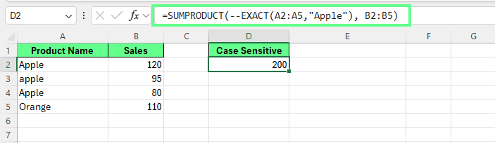
Combining SUMPRODUCT() with EXACT(). Image by Author.

Using VLOOKUP() with SUMPRODUCT()

SUMPRODUCT() can also evaluate lookup results as part of its logic. When combined with VLOOKUP(), it allows conditional calculations based on values stored in a separate table:

=SUMPRODUCT(
  (VLOOKUP(A2:A5, D2:E5, 2, FALSE)="Fruit") *
  B2:B5
)

Here, VLOOKUP() retrieves the category for each product, and SUMPRODUCT() includes only rows that match the specified condition. This approach avoids helper columns and supports more flexible lookup-based filtering than traditional SUMIF() formulas.

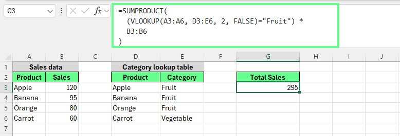
Combining SUMPRODUCT() with VLOOKUP(). Image by Author.

Counting unique values using COUNTIF() with SUMPRODUCT()

You can also use SUMPRODUCT() with COUNTIF() to count unique values like this:

=SUMPRODUCT(1/COUNTIF(A2:A6, A2:A6))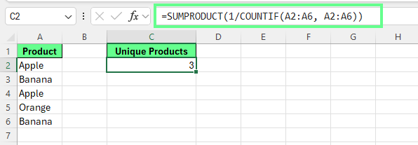

Combining SUMPRODUCT() with COUNTIF(). Image by Author.

In this formula, duplicate values share fractional weights that sum to 1, so each unique item is counted once. That’s why the result is 3. 

While newer functions exist, this technique is still helpful in older versions of Excel or complex array models.

Troubleshooting, Optimization, and Best Practices

Now that you know how and where to use SUMPRODUCT(), here are a few challenges that you may come across and how to solve them: 

Error handling and common challenges

Most SUMPRODUCT() errors come from minor structural issues rather than flawed logic. When a formula returns 0, an unexpected total, or an error, the problem is usually easy to isolate:

Mismatched array sizes

Every array used in SUMPRODUCT() must have the same number of rows and columns. If one range is longer or wider than the others, the formula cannot evaluate correctly.

Quick check: Confirm that all referenced ranges start and end on the same rows and columns.

Unexpected text or hidden characters

SUMPRODUCT() performs numeric math. If a range looks numeric but contains spaces or text, the calculation may return incorrect results or zero.

Quick fix: Use TRIM() to remove extra spaces, or wrap values in -- to force numeric conversion when appropriate.

Misplaced parentheses

Parentheses control evaluation order. A missing or misplaced parenthesis can cause a condition to apply incorrectly or not at all.

Quick fix: Group each logical test clearly before combining it with arithmetic or other conditions.

Test intermediate logic step by step

One of the fastest ways to debug a SUMPRODUCT() formula is to evaluate individual components.

Here’s how you can do this: 

• Highlight a portion of the formula, such as (A2:A10>50)
• Press F9
• Check the output

A healthy condition returns a clean array of TRUE and FALSE values or 1s and 0s if converted. If you see errors or unexpected results, that segment is the source of the issue.

Practical debugging workflow

When a SUMPRODUCT() formula doesn’t behave as expected:

1. Verify array sizes match
2. Confirm numeric ranges contain only numbers
3. Test each condition independently
4. Rebuild the formula incrementally

This approach usually resolves issues quickly without rewriting the entire formula or adding helper columns.

Performance optimization

SUMPRODUCT() evaluates every cell in every referenced array, so the formula structure has a direct impact on performance in large workbooks. But a few choices can prevent slowdowns:

Limit calculation ranges

Avoid whole-column references such as A:A. Instead, restrict formulas to the smallest range necessary: A2:A500. 

Smaller ranges reduce the number of cells SUMPRODUCT() must process and improve recalculation speed.

Simplify logical expressions

Each logical test inside SUMPRODUCT() is evaluated row by row. So, try to combine or streamline conditions where possible, as this reduces the total number of operations.

If two conditions can be expressed as one cleaner rule, performance improves without changing results.

Use structured tables or dynamic named ranges

Excel tables and dynamic named ranges automatically adjust as data grows while keeping ranges tightly scoped. This maintains performance without requiring you to edit formulas as datasets expand.

Be mindful of large arrays

Every additional array and condition increases the calculation workload. In large models, avoid unnecessary criteria and remove arrays that do not directly affect the result.

Working with Excel 365 dynamic arrays

In Excel 365, SUMPRODUCT() does not produce spilled results, but it works reliably with spilled arrays created by functions like FILTER() or UNIQUE(). This allows you to combine dynamic array outputs with SUMPRODUCT() while keeping calculations stable and predictable.

For large, spill-heavy models, consider whether a dynamic array function can replace part of the logic. But when row-by-row multiplication and conditional weighting are required, SUMPRODUCT() is the better option.

Comparing SUMPRODUCT() to Alternative Functions 

SUMPRODUCT() overlaps with several Excel functions, but it solves problems differently. Let’s see how: 

SUMPRODUCT() vs. SUMIF() / SUMIFS()

SUMIF() and SUMIFS() are fast and efficient for straightforward conditions. They work best when:

• Criteria are simple
• Matches are exact
• Logic is strictly AND-based

SUMPRODUCT() trades some speed for flexibility. It’s better suited when calculations require:

• Partial text matches
• OR logic or mixed conditions
• Calculated criteria instead of static ranges
• Complex logic without helper columns

For large datasets with simple rules, SUMIFS() is usually faster. But when precision and control matter more than raw speed, SUMPRODUCT() is the better choice.

SUMPRODUCT() vs. classic array formulas

Traditional array formulas perform many of the same calculations, but they require Ctrl+Shift+Enter (CSE) and can be harder to maintain.

SUMPRODUCT() avoids CSE entirely and behaves like a standard Excel function. This makes formulas easier to read, edit, and share in collaborative or business environments where users may not recognize array formulas.

SUMPRODUCT() vs. modern dynamic array functions

Newer functions such as FILTER(), UNIQUE(), and BYROW() are great at returning spilled results, reshaping data, and producing visible lists or tables.

But SUMPRODUCT() remains valuable when:

• You need a single numeric result
• Logic must stay contained in one cell
• Calculations rely on row-by-row multiplication and weighting
• Backward compatibility matters

Dynamic arrays often complement SUMPRODUCT() rather than replace it, for example, by generating filtered arrays that SUMPRODUCT() then evaluates.

When SUMPRODUCT() is the right choice

Use SUMPRODUCT() when you need:

• Conditional totals with complex logic

• OR conditions or calculated criteria

• Weighted calculations without helper columns

• A single, stable result cell

Implementation across platforms

The core logic behind SUMPRODUCT(): filter, multiply, then sum, is consistent across tools. What changes is how each platform handles logical values and arrays.

Excel vs. Google Sheets behavior

Both Excel and Google Sheets support SUMPRODUCT(), but they differ slightly in how they treat logical values.

In Excel, logical expressions return TRUE and FALSE, which must be explicitly converted into 1 and 0 using the double unary -- or numeric coercion. Without this conversion, calculations may return unexpected results.

Google Sheets handles this conversion automatically. Logical values are treated as numeric (TRUE = 1, FALSE = 0), so SUMPRODUCT() formulas may work without additional operators.

Conceptually, the logic is identical. The difference only lies in whether numeric conversion is implicit or explicit.

Translating SUMPRODUCT() logic to Python

The same pattern applies in Python-based tools such as NumPy or pandas, even though the syntax is different.

In Python, conditions are evaluated row by row and produce Boolean arrays (True and False). These Boolean values already behave like 1 and 0 in calculations, which eliminates the conversion step.

The conceptual flow remains the same:

1. Evaluate a condition
2. Create a Boolean mask
3. Multiply values by that mask
4. Sum the results

Considerations for cross-platform teams

If you or your team works across Excel, Google Sheets, and Python, align on a few key behaviors:

• Boolean logic is the common language: All platforms use TRUE/FALSE-style logic that can be treated as numeric masks.

• Masking replaces helper columns: Excel uses --(condition). Python uses Boolean masks directly.

• Text-matching rules differ: Excel functions like SEARCH() are case-insensitive by default, whereas Python text matching can be case-sensitive depending on configuration.

• Missing values behave differently: Excel blanks and Python NaN values may affect results unless handled consistently.

Across platforms, the key idea stays the same: SUMPRODUCT() represents a reusable calculation pattern.

Final Thoughts

If you want to get better at SUMPRODUCT(), take one real report you already use and rebuild a complex formula without helper columns. That’s how you’ll understand the pattern and see where SUMPRODUCT() may fit in your workflow.

If you want to go further, check out the Data Analysis with Excel Power Tools skills track to see how functions like SUMPRODUCT() fit into broader analytical workflows.