Self-Organizing Maps: An Intuitive Guide with Python Examples

Setting Up the Environment for SOM

Before building the SOM, we need to prepare the environment with the necessary packages. 

Installing Python libraries 

We need these packages: 

• MiniSom is a NumPy-based Python tool that creates and trains SOMs. 
• NumPy is used to access mathematical functions such as splitting arrays, getting unique values, etc. 
• matplotlib is used to plot various graphs and charts to visualize the data. 
• The datasets package from sklearn is used to import datasets on which to apply the SOM. 
• The MinMaxScaler package from sklearn normalizes the dataset. 

The following code snippet imports these packages: 

from minisom import MiniSom
import numpy as np
import matplotlib.pyplot as plt
from sklearn import datasets
from sklearn.preprocessing import MinMaxScaler

Preparing the dataset

In this tutorial, we use MiniSom to build a SOM and then train it on the canonical IRIS dataset. This dataset consists of 3 classes of iris plants. Each class has 50 instances. To prepare the data, we follow these steps: 

• Import the Iris dataset from sklearn, 
• Extract the data vectors and the target scalars. 
• Normalize the data vectors. In this tutorial, we use the MinMaxScaler from scikit-learn. 
• Declare a set of labels for each of the three classes of Iris plants. 

The following code implements these steps: 

dataset_iris = datasets.load_iris()
data_iris = dataset_iris.data
target_iris = dataset_iris.target
data_iris_normalized = MinMaxScaler().fit_transform(data_iris)
labels_iris = {1:'1', 2:'2', 3:'3'}
data = data_iris_normalized
target = target_iris

Implementing Self-Organizing Maps (SOM) in Python

To implement a SOM in Python, we define and initialize the grid before training it on the dataset. We can then visualize the trained neurons and the clustered dataset. 

Defining the SOM grid

As explained earlier, a SOM is a grid of neurons. Using MiniSom, we can create 2-dimensional grids. The grid’s X and Y dimensions are the number of neurons along each axis. To define the SOM grid, we also need to specify:

• The X and Y dimensions of the grid
• The number of input variables - this is the number of data rows. 

Declare these parameters as Python constants:

SOM_X_AXIS_NODES  = 8
SOM_Y_AXIS_NODES  = 8
SOM_N_VARIABLES  = data.shape[1]

The sample code below illustrates how to declare the grid using MiniSom:

som = MiniSom(SOM_X_AXIS_NODES, SOM_Y_AXIS_NODES, SOM_N_VARIABLES)

The first two parameters are the number of neurons along the X and Y axes, and the third parameter is the number of variables. 

We declare other parameters and hyperparameters while creating the SOM grid. We will explain these later in the tutorial. For now, declare these parameters as shown below: 

ALPHA = 0.5
DECAY_FUNC = 'linear_decay_to_zero'
SIGMA0 = 1.5
SIGMA_DECAY_FUNC = 'linear_decay_to_one'
NEIGHBORHOOD_FUNC = 'triangle'
DISTANCE_FUNC = 'euclidean'
TOPOLOGY = 'rectangular'
RANDOM_SEED = 123

Create a SOM using these parameters:

som = MiniSom(
        SOM_X_AXIS_NODES,
        SOM_Y_AXIS_NODES,
        SOM_N_VARIABLES,
        sigma=SIGMA0,
        learning_rate=ALPHA,
        neighborhood_function=NEIGHBORHOOD_FUNC,
        activation_distance=DISTANCE_FUNC,
        topology=TOPOLOGY,
        sigma_decay_function = SIGMA_DECAY_FUNC,
        decay_function = DECAY_FUNC,
        random_seed=RANDOM_SEED,
        )

Initializing the neurons

The above command creates a SOM with random weights for all the neurons. Initializing the neurons with weights drawn from the data (instead of random numbers) can make the training process more efficient. 

When using MiniSom to create a Self-Organizing Map (SOM), there are two ways to initialize the neurons’ weights based on the data:

• Random initialization: The neurons' initial weights are randomly drawn from the input data. We do this by applying the .random_weights_init() function to the SOM. 
• PCA initialization: Principal Component Analysis (PCA) initialization uses the principal components of the input data to initialize the weights. The initial weights of the neurons span the first two principal components. This often leads to faster convergence. 

In this guide, we use PCA initialization. To apply PCA initialization on the SOM weights, use the .pca_weights_init() function as shown below:

som.pca_weights_init(data)

Training the SOM

The training process updates the SOM weights to minimize the distance between the neurons and the data points. 

Below, we explain the iterative training process:

• Initialization: The weight vectors of all the neurons are initialized, typically with random values. It is also possible to initialize the weights by sampling the input data distribution.
• Input selection: An input vector is (randomly) selected from the training dataset.
• BMU identification: The neuron with the weight vector closest to the input vector is identified as the BMU. 
• Neighborhood update: The BMU and its neighboring neurons update their weight vectors. The learning rate and the neighborhood function decide which neurons are updated and by how much. At the iteration step t, given the input vector x, the weight vector of neuron i as w_i, the learning rate (t), and the neighborhood function h_bi (this function quantifies the extent of update for the neuron i given the BMU neuron b), the weight update formula for neuron i is expressed as:
• Decay rate of learning rate and neighborhood radius: Both the learning rate and the neighborhood radius decrease over time. In the earlier iterations, the training process makes larger adjustments over a larger neighborhood. Later iterations help to fine-tune the weights by making smaller changes to the weights of adjacent neurons. This allows the map to stabilize and converge. 

To train the SOM, we present the model with the input data. We can choose from one of two approaches to do this: 

• Pick samples at random from the input data. The .train_random() function implements this technique. 
• Sequentially run through the vectors in the input data. This is done using the .train_batch() function. 

These functions accept the input data and the number of iterations as parameters. In this guide, we use the .train_random() function. Declare the number of iterations as a constant and pass it to the training function: 

N_ITERATIONS = 5000
som.train_random(data, N_ITERATIONS, verbose=True)  

After executing the script and completing the training, a message with the quantization error is displayed:

quantization error: 0.05357240680504421 

The quantization error indicates the amount of information lost when the SOM quantizes (reduces the dimensionality of) the data. A large quantization error indicates a larger distance between the neurons and the data points. It also means that the clustering is less reliable. 

Visualizing SOM neurons 

We now have a trained SOM model. To visualize it, we use a distance map (also known as a U-matrix). The distance map displays the SOM’s neurons as a grid of cells. The color of each cell represents its distance from the neighboring neurons. 

The distance map is a grid with the same dimensions as the SOM. Each cell in the distance map is the normalized sum of the (Euclidean) distances between a neuron and its neighbors. 

Access the SOM distance map using the .distance_map() function. To generate the U-matrix, we follow these steps:

• Use pyplot to create a figure with the same dimensions as the SOM. In this example, the dimensions are 8x8. 
• Plot the distance map using matplotlib using the .pcolor() function. In this example, we use gist_yarg as the color scheme. 
• Display the colorbar, an index mapping different colors to different scalar values. In this case, since the distances are normalized, the scalar distance values range from 0 to 1. 

The code below implements these steps: 

# create the grid
plt.figure(figsize=(8, 8))
#plot the distance map
plt.pcolor(som.distance_map().T, cmap='gist_yarg') 
# show the color bar
plt.colorbar()
plt.show()

In this example, the U-matrix uses a monotone color scheme. It can be understood using these guidelines:

• Lighter shades represent closely spaced neurons, and darker shades represent neurons farther away from others. 
• Groups of lighter shades can be interpreted as clusters. Dark nodes between the clusters can be interpreted as the boundaries between clusters. 

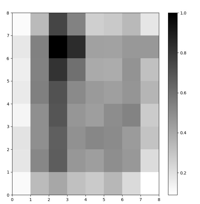
Figure 1: U-matrix of SOM trained on the Iris dataset (image by author)

Evaluating the SOM Clustering Results

The previous figure graphically illustrated the SOM’s neurons. In this section, we show how to visualize how the SOM clustered the data. 

Identifying clusters

We overlay markers over the above U-matrix to denote which class of Iris plant each cell (neuron) represents. To do this:

• As before, create an 8x8 figure using pyplot, plot the distance map, and show the color bar. 
• Specify an array of three matplotlib markers, one for each class of Iris plant. 
• Specify an array of three matplotlib color codes, one for each class of Iris plant. 
• Iteratively plot the winning neuron for each data point:
• Determine the (coordinates of the) winning neuron for each data point using the .winner() function. 
• Plot the position of each winning neuron in the middle of each cell on the grid. w[0] and w[1] give the neuron’s X and Y coordinates, respectively. A value of 0.5 is added to each coordinate to plot it in the middle of the cell. 

The code below shows how to do this:

# plot the distance map
plt.figure(figsize=(8, 8))
plt.pcolor(som.distance_map().T, cmap='gist_yarg') 
plt.colorbar()
# create the markers and colors for each class
markers = ['o', 'x', '^']
colors = ['C0', 'C1', 'C2']
# plot the winning neuron for each data point
for count, datapoint in enumerate(data):
    # get the winner
    w = som.winner(datapoint)  
    # place a marker on the winning position for the sample data point
    plt.plot(w[0]+.5, w[1]+.5, markers[target[count]-1], markerfacecolor='None',
             markeredgecolor=colors[target[count]-1], markersize=12, markeredgewidth=2)
plt.show()

The resulting image is shown below: 

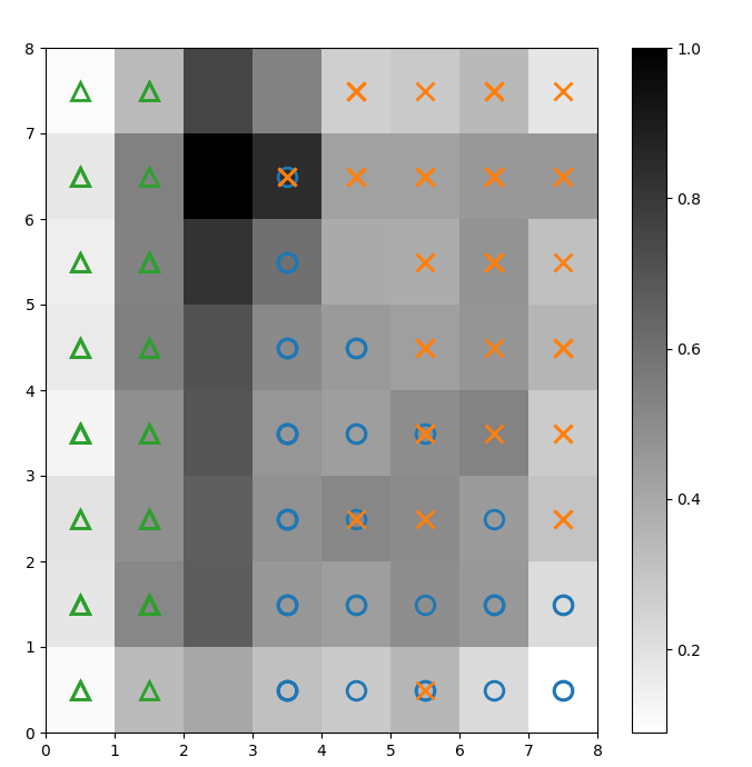
Figure 2: U-matrix overlaid with class markers (image by author)

Based on the Iris dataset documentation, “one class is linearly separable from the other 2; the latter are not linearly separable from each other”. In the U-matrix above, these three classes are represented by three markers - triangle, circle, and cross. 

Notice that there isn’t a clear boundary between the blue circles and the orange crosses. Furthermore, two classes are overlaid on the same neuron in many cells. This means the neuron is equidistant from both classes. 

Visualizing the clustering outcome

A SOM is a clustering model. Similar data points map to the same neuron. Datapoints of the same class map to a cluster of neighboring neurons. We plot all the data points on the SOM grid to better study the clustering behavior. 

The following steps describe how to create this scatter plot:

• Get the winning neuron’s X and Y coordinates of the winning neuron for each data point. 
• Plot the distance map, as we did for Figure 1. 
• Use plt.scatter() to make a scatter plot of all the winning neurons for each data point. Add a random offset to each point to avoid overlaps between data points within the same cell.

We implement these steps in the code below: 

# get the X and Y coordinates of the winning neuron for each data pointw_x, w_y = zip(*[som.winner(d) for d in data])
w_x = np.array(w_x)
w_y = np.array(w_y)
# plot the distance map
plt.figure(figsize=(8, 8))
plt.pcolor(som.distance_map().T, cmap='gist_yarg', alpha=.2)
plt.colorbar()
# make a scatter plot of all the winning neurons for each data point
# add a random offset to each point to avoid overlaps
for c in np.unique(target):
    idx_target = target==c
    plt.scatter(w_x[idx_target]+.5+(np.random.rand(np.sum(idx_target))-.5)*.8,
                w_y[idx_target]+.5+(np.random.rand(np.sum(idx_target))-.5)*.8,
                s=50, 
                c=colors[c-1], 
                label=labels_iris[c+1]
                )
plt.legend(loc='upper right')
plt.grid()
plt.show()

The following graph shows the output scatter plot:

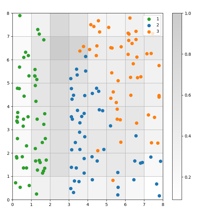
Figure 3: Scatter plot of data points within cells (image by author)

In the above scatter plot, observe that: 

• Some cells contain both blue and orange dots. 
• The green dots are clearly separated from the rest of the data, but the blue and orange dots are not cleanly separated. 
• The above observations align with the fact that only one of the three clusters in the Iris dataset has a clear boundary. 
• In Figure 1, dark nodes between the clusters (which can be interpreted as the boundaries between clusters) match with empty cells in the scatter plot. 

You can access and run the complete code on this DataLab notebook. 

Tuning the SOM Model

The previous sections showed how to create and train a SOM model and how to study the results visually. In this section, we discuss how to tune the performance of SOM models. 

Key hyperparameters to tune

As with any machine learning model, hyperparameters considerably impact the model’s performance. 

Some of the hyperparameters important in training SOMs are:

• The grid size decides the map’s size. The number of neurons in a map with a grid size of AxB is A*B. 
• The learning rate decides how much the weights are changed in each iteration. We set the initial learning rate, and it decreases over time according to the decay function. 
• The decay function decides the extent to which the learning rate is decreased in each subsequent iteration. 
• The neighborhood function is a mathematical function that specifies which neurons are to be considered as the BMU’s neighbors. 
• The standard deviation specifies the neighborhood function’s spread. For example, a Gaussian neighborhood function with a high standard deviation will have a larger neighborhood than the same function with a smaller standard deviation. We set the initial standard deviation, which decreases over time according to the sigma decay function. 
• The sigma decay function controls how much the standard deviation is reduced in each subsequent iteration. 
• The number of training iterations decides how many times the weights are updated. In each training iteration, the neuron weights are updated once. 
• The distance function is a mathematical function that calculates the distance between neurons and data points. 
• The topology decides the grid structure’s layout. The neurons in the grid can be arranged in a rectangular or hexagonal pattern. 

In the next section, we discuss guidelines for setting the values of these hyperparameters. 

Impact of hyperparameter tuning

Hyperparameter values should be decided based on the model and the dataset. To some extent, determining these values is a process of trial and error. In this section, we give guidelines for tuning each hyperparameter. Next to each hyperparameter, we mention (in parentheses) the respective Python constants used in the sample code.

• Grid size (SOM_X_AXIS_NODES and SOM_Y_AXIS_NODES): The grid size depends on the dataset’s size. The rule of thumb is that given a dataset of size N, the grid should contain roughly 5*sqrt(N) neurons. For example, if the dataset has 150 samples, the grid should contain 5*sqrt(150) = approximately 61 neurons. In this tutorial, the Iris dataset has 150 rows and we use an 8x8 grid. 
• Initial learning rate (ALPHA): A higher rate speeds up convergence, while lower rates are used for finer adjustments after early iterations. The initial learning rate should be large enough to enable quick adaptation but not so large that it overshoots optimal weight values. In this article, the initial learning rate is 0.5. 
• Initial standard deviation (SIGMA0): It determines the neighborhood’s initial size or spread. A larger value considers more global patterns. In this example, we use a starting standard deviation of 1.5. 
• For the decay rate (DECAY_FUNC) and the sigma decay rate (SIGMA_DECAY_FUNC), we can choose from one of three types of decay functions: 
• Inverse decay: This function is suitable if the data has both global and local patterns. In such cases, we need a longer phase of broad learning before focusing on local patterns. 
• Linear decay: This is good for datasets where we want a steady and uniform neighborhood size or learning rate reduction. This is useful if the data doesn't need much fine-tuning.
• Asymptotic decay: This function is useful if the data is complex and high-dimensional. In such cases, it is better to spend more time on global exploration before gradually transitioning to finer details. 
• Neighborhood function (NEIGHBORHOOD_FUNC): The default choice of the neighborhood function is the Gaussian function. Other functions, as explained below, are also used. 
• Gaussian (default): This is a bell-shaped curve. The extent to which a neuron is updated decreases smoothly as its distance from the winning neuron increases. It provides a smooth and continuous transition and preserves the data’s topology. It is suitable for most general purposes due to its stable and predictable behavior.
• Bubble: This function creates a fixed-width neighborhood. All neurons within this neighborhood are updated equally, and neurons outside this neighborhood are not updated (for a given data point). It is computationally cheaper and easier to implement. It is useful for smaller maps where sharp neighborhood boundaries do not compromise effective clustering. 
• Mexican hat: It has a central positive region surrounded by a negative region. Neurons close to the BMU are updated to come closer to the data point, and neurons further away are updated to move away from the data point. This technique enhances contrast and sharpens the features in the map. Since it emphasizes distinct clusters, it is effective in pattern recognition tasks where a clear separation of clusters is desired.
• Triangle: This function defines the neighborhood size as a triangle, with the BMU having the largest influence. It decreases linearly with distance from the BMU. It is used for clustering data with gradual transitions between clusters or features, such as image, speech, or time-series data, where neighboring data points are expected to share similar characteristics. 
• Distance function (DISTANCE_FUNC): To measure the distance between neurons and data points, we can choose from 4 methods:
• Euclidean distance (default choice): Useful when the data is continuous, and we want to measure straight-line distance. It suits most general tasks, especially when data points are evenly distributed and spatially related.
• Cosine distance: Good choice for text or high-dimensional sparse data where the angle between vectors is more important than magnitude. It’s useful for comparing directionality in data.
• Manhattan distance: Ideal when data points are on a grid or lattice (e.g., city blocks). This is less sensitive to outliers than Euclidean distance.
• Chebyshev distance: Suitable for situations where movement can occur in any direction (e.g., chessboard distances). It is useful for discrete spaces where we want to prioritize the maximum axis difference.
• Topology (TOPOLOGY): In a grid, neurons can be arranged in a hexagonal or rectangular structure: 
• Rectangular (default): each neuron has 4 immediate neighbors. This is the right choice when the data doesn’t have a clear spatial relationship. It is also computationally simpler. 
• Hexagonal: each neuron has 6 neighbors. This is the preferred option if the data has spatial relationships better represented with a hexagonal grid. This is the case for circular or angular data distributions.
• Number of training iterations (N_ITERATIONS): In principle, longer training times lead to lower errors and better alignment of the weights with the input data. However, the model’s performance increases asymptotically with the number of iterations. Thus, after a certain number of iterations, the performance increase from subsequent interactions is only marginal. Deciding the correct number of iterations takes some experimentation. In this tutorial, we train the model over 5000 iterations. 

To determine the right configuration of hyperparameters, we recommend experimenting with various options on a smaller subset of the data.

Conclusion

Self-organizing maps are a robust tool for unsupervised learning. They are used for clustering, dimensionality reduction, anomaly detection, and data visualization. Since they preserve the topological properties of high-dimensional data and represent it on a lower-dimensional grid, SOMs make it easy to visualize and interpret complex datasets. 

This tutorial discussed the underlying principles of SOMs and showed how to implement a SOM using the MiniSom Python library. It also demonstrated how to visually analyze the results and explained the important hyperparameters used to train SOMs and finetune their performance.