Variational Autoencoders: How They Work and Why They Matter

As machine learning technology advances at an unprecedented pace, Variational Autoencoders (VAEs) are revolutionizing the way we process and generate data. By merging powerful data encoding with innovative generative capabilities, VAEs offer transformative solutions to complex challenges in the field.

In this article, we'll explore the core concepts behind VAEs, their applications, and how they can be effectively implemented using PyTorch, step-by-step.

What is a Variational Autoencoder?

Autoencoders are a type of neural network designed to learn efficient data representations, primarily for the purpose of dimensionality reduction or feature learning. 

Autoencoders consist of two main parts: 

1. The encoder: Compresses the input data into a lower-dimensional latent space.
2. The decoder: Reconstructs the original data from this compressed representation. 

The primary objective of autoencoders is to minimize the difference between the input and the reconstructed output, thus learning a compact representation of the data.

Enter Variational Autoencoders (VAEs), which extend the capabilities of the traditional autoencoder framework by incorporating probabilistic elements into the encoding process. 

While standard autoencoders map inputs to fixed latent representations, VAEs introduce a probabilistic approach where the encoder outputs a distribution over the latent space, typically modeled as a multivariate Gaussian. This allows VAEs to sample from this distribution during the decoding process, leading to the generation of new data instances.

The key innovation of VAEs lies in their ability to generate new, high-quality data by learning a structured, continuous latent space. This is particularly important for generative modeling, where the goal is not just to compress data but to create new data samples that resemble the original dataset. 

VAEs have demonstrated significant effectiveness in tasks such as image synthesis, data denoising, and anomaly detection, making them relevant tools for advancing the capabilities of machine learning models and applications.

Variational Autoencoders Theoretical Background

In this section, we will introduce the theoretical background and operational mechanics of VAEs, providing you with a solid base for exploring their applications in later sections.

Let’s start with encoders. The encoder is a neural network responsible for mapping input data to a latent space. Unlike traditional autoencoders that produce a fixed point in the latent space, the encoder in a VAE outputs parameters of a probability distribution—typically the mean and variance of a Gaussian distribution. This allows the VAE to model data uncertainty and variability effectively.

Another neural network called a decoder is used to reconstruct the original data from the latent space representation. Given a sample from the latent space distribution, the decoder aims to generate an output that closely resembles the original input data. This process allows the VAE to create new data instances by sampling from the learned distribution.

The latent space is a lower-dimensional, continuous space where the input data is encoded.

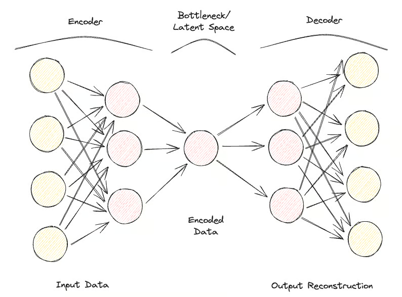
Visualization of the role of the encoder, decoder, and latent space. Image source.

The variational approach is a technique used to approximate complex probability distributions. In the context of VAEs, it involves approximating the true posterior distribution of latent variables given the data, which is often intractable. 

The VAE learns an approximate posterior distribution. The goal is to make this approximation as close as possible to the true posterior.

Bayesian inference is a method of updating the probability estimate for a hypothesis as more evidence or information becomes available. In VAEs, Bayesian inference is used to estimate the distribution of latent variables. 

By integrating prior knowledge (prior distribution) with the observed data (likelihood), VAEs adjust the latent space representation through the learned posterior distribution.

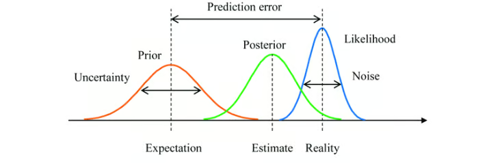
Bayesian inference with a prior distribution, posterior distribution, and likelihood function. Image source.

Here is how the process flow looks:

1. The input data x is fed into the encoder, which outputs the parameters of the latent space distribution q(z∣x) (mean μ and variance σ²).
2. Latent variables z are sampled from the distribution q(z∣x) using techniques like the reparameterization trick.
3. The sampled z is passed through the decoder to produce the reconstructed data x̂, which should be similar to the original input x.

Variational Autoencoder vs Traditional Autoencoder

Let’s examine the differences and advantages of VAEs over traditional autoencoders.

Architecture comparison

As seen before, traditional autoencoders consist of an encoder network that maps the input data x to a fixed, lower-dimensional latent space representation z. This process is deterministic, meaning each input is encoded into a specific point in the latent space. 

The decoder network then reconstructs the original data from this fixed latent representation, aiming to minimize the difference between the input and its reconstruction. 

Traditional autoencoders' latent space is a compressed representation of the input data without any probabilistic modeling, which limits their ability to generate new, diverse data since they lack a mechanism to handle uncertainty.

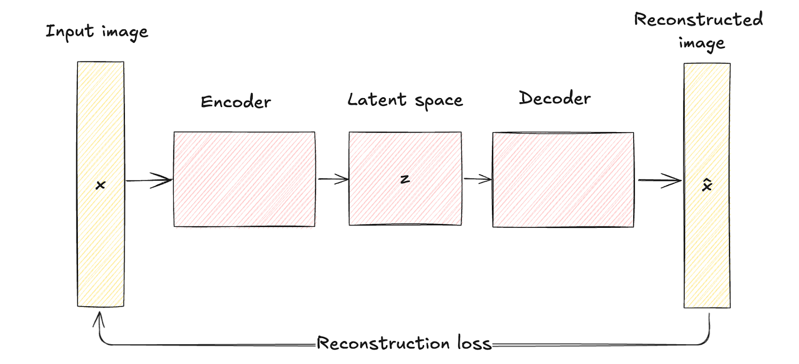
Autoencoder architecture. Image by author

VAEs introduce a probabilistic element into the encoding process. Namely, the encoder in a VAE maps the input data to a probability distribution over the latent variables, typically modeled as a Gaussian distribution with mean μ and variance σ².

This approach encodes each input into a distribution rather than a single point, adding a layer of variability and uncertainty.

Architectural differences are visually represented by the deterministic mapping in traditional autoencoders versus the probabilistic encoding and sampling in VAEs.

This structural difference highlights how VAEs incorporate regularization through a term known as KL divergence, shaping the latent space to be continuous and well-structured. 

The regularization introduced significantly enhances the quality and coherence of the generated samples, surpassing the capabilities of traditional autoencoders.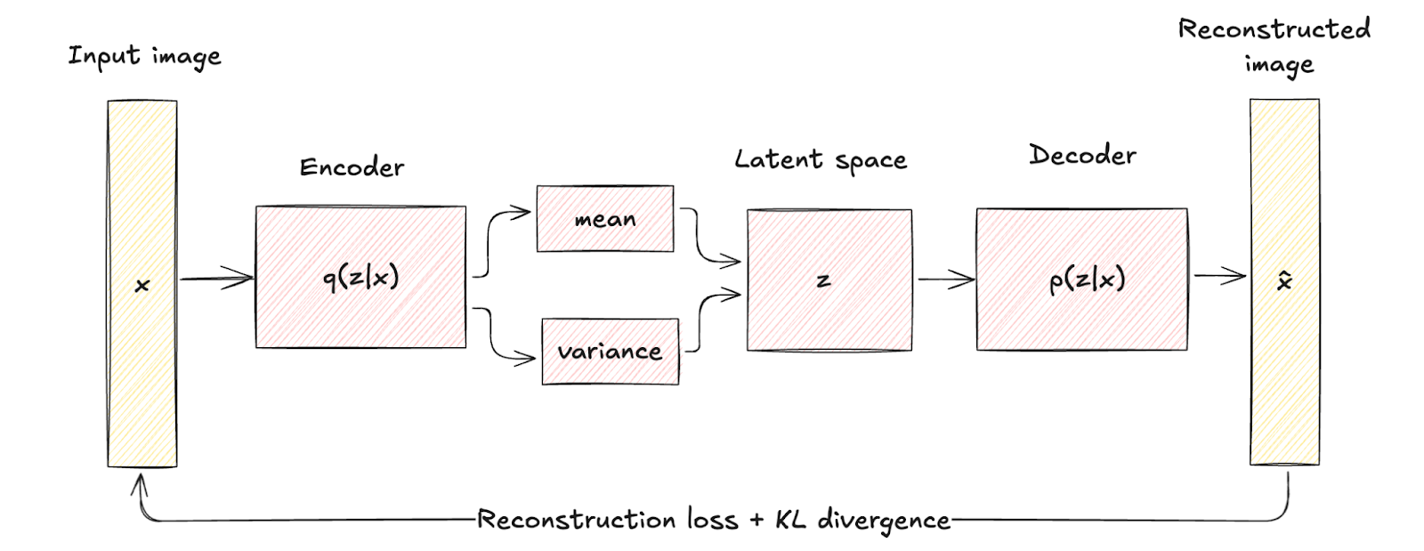

Variational Autoencoder architecture. Image by author

Applications comparison

VAEs' probabilistic nature significantly expands their range of applications compared to that of traditional autoencoders. In contrast, traditional autoencoders are highly effective in applications where deterministic data representation is sufficient. 

Let’s take a look at a few applications of each to better drive this point home. 

Applications of VAEs

• Generative modeling. The core advantage of VAEs is their ability to generate new data samples that are similar to the training data but not identical to any specific instance. For example, in image synthesis, VAEs can create new images that resemble the training set but with variations, making them useful for tasks like creating new artwork, generating realistic faces, or producing new designs in fashion and architecture.
• Anomaly detection. By learning the distribution of normal data, VAEs can identify deviations from this distribution as anomalies. This is particularly useful in applications like fraud detection, network security, and predictive maintenance.
• Data imputation and denoising. One of VAEs' strong points is reconstructing data with missing or noisy parts. By sampling from the learned latent distribution, they are able to predict and fill in missing values or remove noise from corrupted data. This makes them valuable in applications such as medical imaging, where accurate data reconstruction is essential, or in restoring corrupted audio and visual data.
• Semi-supervised learning. In semi-supervised learning scenarios, VAEs can improve classifier performance by using the latent space to capture underlying data structures, thereby enhancing the learning process with limited labeled data.
• Latent space manipulation. VAEs provide a structured and continuous latent space that can be manipulated for various applications. For instance, in image editing, specific features (like lighting or facial expressions) can be adjusted by navigating the latent space. This feature is particularly useful in creative industries for modifying and enhancing images and videos.

Applications of traditional autoencoders

• Dimensionality reduction. Traditional autoencoders are widely used to reduce the dimensionality of data. By encoding data into a lower-dimensional latent space and then reconstructing it, they can capture the most important features of the data. This is useful in scenarios such as data visualization, where high-dimensional data needs to be projected into two or three dimensions, and in preprocessing steps for other machine learning models to improve performance and reduce computational costs.
• Feature extraction. By training the encoder to capture the essential aspects of the input data, the latent representations can be used as compact feature vectors for downstream tasks like classification, clustering, and regression. This is particularly beneficial in applications such as image recognition, where the latent space can reveal important visual patterns.
• Denoising. Traditional autoencoders are effective in denoising data by learning to reconstruct clean inputs from noisy versions. This application is valuable in scenarios such as image processing, where removing noise from images can enhance visual quality, and in signal processing, where it can improve the clarity of audio signals.
• Data compression. The compact latent vectors can be stored or transmitted more efficiently than the original high-dimensional data, and the decoder can reconstruct the data when needed. This is particularly useful in applications like image and video compression.
• Image reconstruction and inpainting. Traditional autoencoders can be used to reconstruct missing parts of images. In image inpainting, the autoencoder is trained to fill in missing or corrupted regions of an image based on the context provided by the surrounding pixels. This is useful in fields like computer vision and digital restoration.
• Sequence learning. Autoencoders can be adapted to work with sequential data using recurrent or convolutional layers. They can capture temporal dependencies and patterns, making them useful for applications like text generation, speech synthesis, and financial forecasting.

Types of Variational Autoencoders

VAEs have evolved into various specialized forms to address different challenges and applications in machine learning. In this section, we’ll examine the most prominent types, highlighting use cases, advantages, and limitations.  

Conditional variational autoencoder

Conditional Variational Autoencoders (CVAEs) are a specialized form of VAEs that enhance the generative process by conditioning on additional information. 

A VAE becomes conditional by incorporating additional information, denoted as c, into both the encoder and decoder networks. This conditioning information can be any relevant data, such as class labels, attributes, or other contextual data.

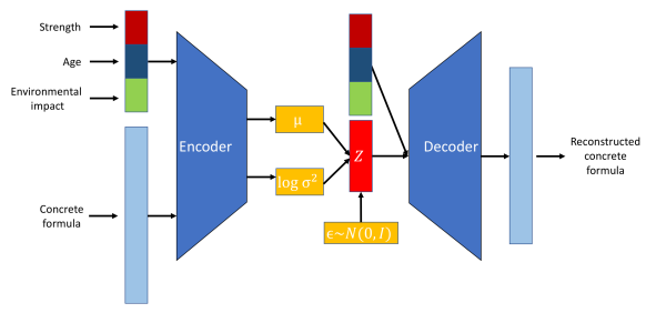
CVAE model structure. Image source.

Use cases of CVAEs include: 

• Controlled data generation. For example, in image generation, a CVAE can create images of specific objects or scenes based on given labels or descriptions.
• Image-to-image translation. CVAEs can transform images from one domain to another while maintaining specific attributes. For instance, they can be used to translate black-and-white images to color images or to convert sketches into realistic photos.
• Text generation. CVAEs can generate text conditioned on specific prompts or topics, making them useful for tasks like story generation, chatbot responses, and personalized content creation.

The pros and cons are: 

• Finer control over generated data 
• Improved representation learning
• Increased risk of overfitting

Other variants

Disentangled Variational Autoencoders, often called Beta-VAEs, are another type of specialized VAEs. They aim to learn latent representations where each dimension captures a distinct and interpretable factor of variation in the data. This is achieved by modifying the original VAE objective with a hyperparameter β that balances the reconstruction loss and the KL divergence term.

Pros and cons of Beta-VAEs: 

• Improved interpretability of latent factors.
• Enhanced ability to manipulate individual features of the generated data.
• Requires careful tuning of the β parameter.
• May result in poorer reconstruction quality if the balance between terms is not optimal.

Another variant of VAEs is Adversarial Autoencoders (AAEs). AAEs combine the VAE framework with adversarial training principles from Generative Adversarial Networks (GANs). An additional discriminator network ensures that the latent representations match a prior distribution, enhancing the model's generative capabilities.

Pros and cons of AAEs:

• Produces high-quality and realistic data samples.
• Effective in regularizing the latent space.
• Increased training complexity due to the adversarial component.
• Potential issues with training stability, similar to GANs.

Now, we will look at two more extensions of Variational Autoencoders.

The first is Variational Recurrent Autoencoders (VRAEs). VRAEs extend the VAE framework to sequential data by incorporating recurrent neural networks (RNNs) into the encoder and decoder networks. This allows VRAEs to capture temporal dependencies and model sequential patterns.

Pros and cons of VRAEs:

• Effective in handling time-series data and sequential patterns.
• Useful in applications like speech synthesis, music generation, and time-series forecasting.
• Higher computational requirements due to the recurrent nature of the model.

The last variant we will examine is Hierarchical Variational Autoencoders (HVAEs). HVAEs introduce multiple layers of latent variables arranged in a hierarchical structure, which allows the model to capture more complex dependencies and abstractions in the data. 

Pros and cons of HVAEs:

• Capable of modeling complex data distributions with hierarchical structures.
• Provides more expressive latent representations.
• Increased model complexity and computational cost.

Implementing a Variational Autoencoder with PyTorch

In this section, we will implement a simple Variational Autoencoder (VAE) using PyTorch.

1. Setting up the environment

To implement a VAE, we need to set up our Python environment with the necessary libraries and tools. The libraries we will use are: 

• PyTorch
• torchvision
• matplotlib
• numpy

Here’s the code to install these libraries: 

pip install torch torchvision matplotlib numpy

2. Implementation

Let's walk through the implementation of a VAE step-by-step. First, we must import the libraries: 

import torch 
import torch.nn as nn 
import torch.optim as optim 
from torchvision import datasets, transforms 
from torch.utils.data import DataLoader 
import matplotlib.pyplot as plt 
import numpy as np

Next, we must define the encoder, decoder, and VAE. Here’s the code: 

class Encoder(nn.Module):
    def __init__(self, input_dim, hidden_dim, latent_dim):
        super(Encoder, self).__init__()
        self.fc1 = nn.Linear(input_dim, hidden_dim)
        self.fc_mu = nn.Linear(hidden_dim, latent_dim)
        self.fc_logvar = nn.Linear(hidden_dim, latent_dim)
        
    def forward(self, x):
        h = torch.relu(self.fc1(x))
        mu = self.fc_mu(h)
        logvar = self.fc_logvar(h)
        return mu, logvar
class Decoder(nn.Module):
    def __init__(self, latent_dim, hidden_dim, output_dim):
        super(Decoder, self).__init__()
        self.fc1 = nn.Linear(latent_dim, hidden_dim)
        self.fc2 = nn.Linear(hidden_dim, output_dim)
        
    def forward(self, z):
        h = torch.relu(self.fc1(z))
        x_hat = torch.sigmoid(self.fc2(h))
        return x_hat
class VAE(nn.Module):
    def __init__(self, input_dim, hidden_dim, latent_dim):
        super(VAE, self).__init__()
        self.encoder = Encoder(input_dim, hidden_dim, latent_dim)
        self.decoder = Decoder(latent_dim, hidden_dim, input_dim)
        
    def forward(self, x):
        mu, logvar = self.encoder(x)
        std = torch.exp(0.5 * logvar)
        eps = torch.randn_like(std)
        z = mu + eps * std
        x_hat = self.decoder(z)
        return x_hat, mu, logvar

We also have to define the loss function. The loss function for VAEs consists of a reconstruction loss and a KL divergence loss. This is how it looks in PyTorch: 

def loss_function(x, x_hat, mu, logvar):
    BCE = nn.functional.binary_cross_entropy(x_hat, x, reduction='sum')
    KLD = -0.5 * torch.sum(1 + logvar - mu.pow(2) - logvar.exp())
    return BCE + KLD

To train the VAE, we will load the MNIST dataset, define the optimizer, and train the model.

# Hyperparameters
input_dim = 784
hidden_dim = 400
latent_dim = 20
lr = 1e-3
batch_size = 128
epochs = 10
# Data loader
transform = transforms.Compose([transforms.ToTensor(), transforms.Lambda(lambda x: x.view(-1))])
train_dataset = datasets.MNIST(root='./data', train=True, transform=transform, download=True)
train_loader = DataLoader(train_dataset, batch_size=batch_size, shuffle=True)
# Model, optimizer
vae = VAE(input_dim, hidden_dim, latent_dim)
optimizer = optim.Adam(vae.parameters(), lr=lr)
# Training loop
vae.train()
for epoch in range(epochs):
    train_loss = 0
    for x, _ in train_loader:
        x = x.view(-1, input_dim)
        optimizer.zero_grad()
        x_hat, mu, logvar = vae(x)
        loss = loss_function(x, x_hat, mu, logvar)
        loss.backward()
        train_loss += loss.item()
        optimizer.step()
    
    print(f"Epoch {epoch + 1}, Loss: {train_loss / len(train_loader.dataset)}")

3. Testing and evaluating the model

After training, we can evaluate the VAE by visualizing the reconstructed outputs and generated samples.

This is the code: 

# visualizing reconstructed outputs
vae.eval()
with torch.no_grad():
    x, _ = next(iter(train_loader))
    x = x.view(-1, input_dim)
    x_hat, _, _ = vae(x)
    x = x.view(-1, 28, 28)
    x_hat = x_hat.view(-1, 28, 28)
    
    fig, axs = plt.subplots(2, 10, figsize=(15, 3))
    for i in range(10):
        axs[0, i].imshow(x[i].cpu().numpy(), cmap='gray')
        axs[1, i].imshow(x_hat[i].cpu().numpy(), cmap='gray')
        axs[0, i].axis('off')
        axs[1, i].axis('off')
    plt.show()
#visualizing generated samples
with torch.no_grad():
    z = torch.randn(10, latent_dim)
    sample = vae.decoder(z)
    sample = sample.view(-1, 28, 28)
    
    fig, axs = plt.subplots(1, 10, figsize=(15, 3))
    for i in range(10):
        axs[i].imshow(sample[i].cpu().numpy(), cmap='gray')
        axs[i].axis('off')
    plt.show()

Visualization of outputs. The top row is the original MNIST data, the middle row is the reconstructed outputs, and the last row is the generated samples—image by author.

Variational Autoencoders Challenges and Solutions

While Variational Autoencoders (VAEs) are powerful tools for generative modeling, they come with several challenges and limitations that can affect their performance. Let’s discuss some of them, and provide mitigation strategies.

Mode collapse

This is a phenomenon where the VAE fails to capture the full diversity of the data distribution. The result is generated samples representing only a few modes (distinct regions) of the data distribution while ignoring others. This leads to a lack of variety in the generated outputs. 

Mode collapse caused by: 

• Poor latent space exploration: If the latent space is not adequately explored during training, the model might only learn to generate samples from a few regions.
• Insufficient training data: Limited or unrepresentative training data can cause the model to overfit to specific modes.

Mode collapse can be mitigated by using: 

• Regularization techniques: Using techniques like dropout and batch normalization can help improve generalization and reduce mode collapse.
• Improved training algorithms: Important-weighted autoencoders (IWAE) can provide better gradient estimates and improve latent space exploration.

Uninformative latent spaces

In some cases, the latent space learned by a VAE might become uninformative, where the model does not effectively use the latent variables to capture meaningful features of the input data. This can result in poor quality of generated samples and reconstructions.

This typically happens because of the following reasons: 

• Imbalanced loss components: The trade-off between the reconstruction loss and the KL divergence might not be well-balanced, causing the latent variables to be ignored.
• Posterior collapse: The encoder learns to output a posterior distribution that is very close to the prior, leading to a loss of information in the latent space.

Uninformative latent spaces can be fixed by leveraging the warm-up strategy, which involves gradually increasing the weight of the KL divergence during training or by directly modifying the weight of the KL divergence term in the loss function. 

Training instability

Training VAEs can sometimes be unstable, with the loss function oscillating or diverging. This can make it difficult to achieve convergence and obtain a well-trained model.

The reason this occurs is because: 

• Complex loss landscape: The VAE loss function combines reconstruction and regularization terms, leading to a complex optimization landscape.
• Hyperparameter sensitivity: VAEs are sensitive to the choice of hyperparameters, such as the learning rate, the weight of the KL divergence, and the architecture of the neural networks.

Steps to mitigate training instability involve either using: 

• Careful hyperparameter tuning: Systematic exploration of hyperparameters can help find stable configurations for training.
• Advanced optimizers: Using adaptive learning rate optimizers like Adam can help navigate the complex loss landscape more effectively.

Computational costs

Training VAEs, especially with large and complex datasets, can be computationally expensive. This is due to the need for sampling and backpropagation through stochastic layers.

The cause of high computational costs include:

• Large networks: The encoder and decoder networks can become large and deep, increasing the computational burden.
• Latent space sampling: Sampling from the latent space and calculating gradients through these samples can add to the computational cost.

These are some mitigation actions:

• Model simplification: Reducing the complexity of the encoder and decoder networks can help reduce computational costs.
• Efficient sampling techniques: Using more efficient sampling methods or approximations can reduce the computational load.

Conclusion

Variational Autoencoders (VAEs) have proven to be a groundbreaking advancement in the realm of machine learning and data generation. 

By introducing probabilistic elements into the traditional autoencoder framework, VAEs enable the generation of new, high-quality data and provide a more structured and continuous latent space. This unique capability has opened up a wide array of applications, from generative modeling and anomaly detection to data imputation and semi-supervised learning.

In this article, we’ve covered the fundamentals of Variational Autoencoders, the different types, how to implement VAEs in PyTorch, as well as challenges and solutions when working with with VAEs.

Check out these resources to continue your learning: 

• Introduction to Deep Learning with Keras
• Introduction to TensorFlow in Python
• PyTorch vs TensorFlow vs Keras
• How Transformers Work: A Detailed Exploration of Transformer Architecture