Laplacian Explained: From Calculus to ML

The Laplacian appears in graph-based algorithms, image processing pipelines, and spectral clustering. So if you're building models that work with graphs, images, or high-dimensional data, the Laplacian isn't optional background math. It's the thing actually doing the work under the hood.

In this article, I'll cover the Laplacian from the ground up: the math behind it, the geometric intuition, the graph Laplacian and its matrix form, and how it ‘s used in real machine learning applications.

Do you need a practical introduction to differential equations? Read our recent article to go from fundamentals to practical machine learning applications.

What Is the Laplacian?

The Laplacian is a second-order differential operator. It tells you how a function curves at any given point.

You’ll sometimes see it described as the divergence of the gradient.

And that’s the key to understanding what the operator actually does:

• The gradient tells you which direction a function increases fastest
• The divergence measures whether that flow spreads out or pulls in.

When combined, the Laplacian tells you whether a point is a local peak, a local valley, or somewhere flat in between.

In plain terms, the Laplacian measures how much a function's value at a point differs from the average value of its neighbors. If the Laplacian is zero, the function is locally "balanced." Positive means the point sits below its surroundings. Negative means it sits above them.

The formula

In 2D, for a function f(x, y):

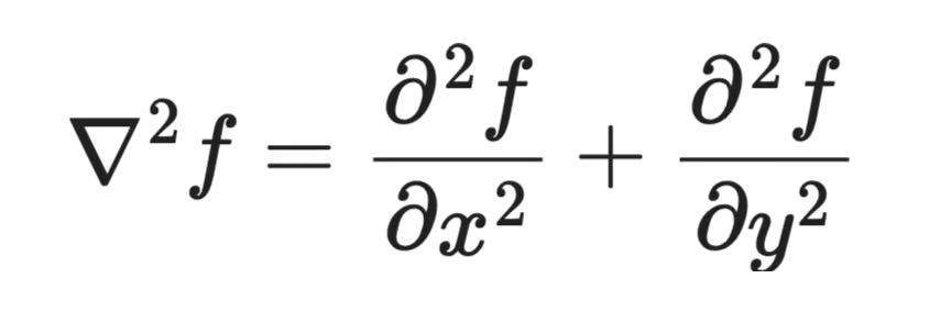
2D Laplacian formula

In 3D, for a function f(x, y, z):

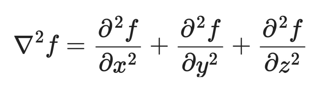
3D Laplacian formula

The pattern holds in any number of dimensions - you sum the second partial derivatives along each axis. This makes the Laplacian a great fit for high-dimensional data, which is exactly why it shows up so often in machine learning.

Laplacian Formula in Multivariable Calculus

The Laplacian formula is shorter than you'd expect for something that shows up across so much of machine learning.

In 3D, for a function f(x, y, z), it looks like this:

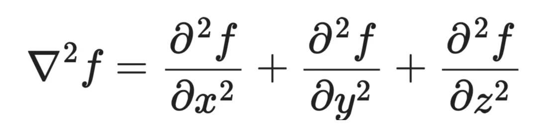
3D Laplacian formula

That's it. You're summing the second partial derivatives along each dimension.

Each term asks the same question along its axis: is the function curving upward, curving downward, or flat? When you add those answers together, you get a single number that describes the overall curvature at that point.

From 3D to n dimensions

The formula generalizes to n dimensions. This is the generic formula for a function with n input dimensions:

Laplacian formula generalization

This is why the Laplacian works well in machine learning, where your data often lives in hundreds or thousands of dimensions. The operator just sums the curvature along each dimension.

Connection to optimization

If you've worked with gradient descent, you already think about first derivatives - which direction is downhill? The Laplacian takes you one step further.

Second derivatives tell you about the shape of that hill.

A large positive Laplacian at a point means the function curves sharply upward in all directions - you're near a minimum. A large negative value means you're near a maximum. Near zero means the surface is locally flat.

This curvature information matters in second-order optimization methods, which use it to take smarter steps than plain gradient descent. The Laplacian is one way to summarize that curvature in a single scalar value.

Geometric Intuition: What the Laplacian Measures

The sign of the Laplacian at a point tells you the shape of the function around it.

• If ∇²f > 0 at a point, the function curves upward in all directions. The point is lower than its surroundings. That's convexity.

• If ∇²f < 0, the function curves downward. The point is higher than its surroundings. That's concavity.

• If ∇²f = 0, the function is locally flat. No net curvature in any direction.

This is the multivariable version of the second derivative test you already know. In 1D, a positive second derivative means a local minimum and a negative one means a local maximum. The Laplacian extends that same idea to any number of dimensions by summing curvature across all axes.

Relationship to the Hessian

The Hessian matrix captures the full curvature picture. It's a matrix of all second partial derivatives, and each entry describes how the function curves along a pair of axes.

The Laplacian is the trace of the Hessian - the sum of its diagonal entries. Where the Hessian gives you the complete curvature breakdown, the Laplacian collapses it into a single number.

That trade-off is important in machine learning. The full Hessian is expensive to compute for high-dimensional models - a model with n parameters has an n × n Hessian. The Laplacian gives you a cheap, scalar summary of curvature that's fast to work with.

Why this matters for machine learning

When you're training a model, you're navigating a loss surface. Flat regions mean slow learning. Convex areas mean the optimizer can overshoot. The Laplacian gives you a quick read on which situation you're in.

Graph-based methods use Laplacian to measure how smoothly values change across a graph's nodes. It’s a direct extension of the same curvature intuition from continuous functions to discrete structures.

Laplacian and Optimization in Machine Learning

Gradient descent only uses first derivatives.

The gradient tells you which direction to step. It doesn't tell you how big that step should be. A steep gradient in a flat, wide valley calls for a big step. The same steep gradient near a sharp cliff edge calls for a small one. First derivatives alone can't tell the difference.

That's where second derivatives come in.

Curvature and step size

Curvature describes how fast the gradient itself is changing. High curvature means the loss surface bends sharply - small steps in parameter space produce large changes in the gradient. Low curvature means the surface is flat and the gradient changes slowly.

If you ignore curvature and use a fixed learning rate, you're guessing. Too large, and you overshoot in high-curvature regions. Too small, and you crawl through flat ones.

Second-order optimization methods like Newton's method use curvature to automatically set step sizes. They divide the gradient by the curvature, taking bigger steps where the surface is flat and smaller steps where it's sharp.

Where the Laplacian fits

The Laplacian is the trace of the Hessian - a single scalar that summarizes the total curvature at a point. It doesn't capture the full picture the way the Hessian does, but it's cheap to compute and useful as a signal.

Here’s a plain English explanation of what you need to remember:

• A large positive Laplacian of the loss at a point means you're near a local minimum - the loss curves upward in all directions
• A negative value means you're near a maximum
• Near zero means you're in a flat or saddle region, which is exactly where gradient descent tends to stall

Stability and regularization

Curvature also connects to training stability. Sharp minima - regions with high curvature - tend to generalize worse than flat ones. A model that converges into a sharp minimum is sensitive to small changes in input.

Some regularization techniques directly penalize curvature to push optimization toward flatter regions of the loss surface. The Laplacian shows up here too, as a way to measure and constrain how sharply the model's predictions change across input space.

Understanding curvature helps you understand why your optimizer stalls, why your learning rate matters so much, and why some minima generalize better than others.

The Graph Laplacian and Laplacian Matrix

So far, the Laplacian has lived in the world of continuous functions. But what happens when your data isn't a smooth surface, but a graph instead?

That's where the graph Laplacian comes in. It takes the same core idea - measuring how a value at one point differs from its neighbors - and applies it to nodes and edges.

The formula

The graph Laplacian L is defined as:

Graph Laplacian formula (simplified)

Two matrices. That's it. Let's break down what each one means.

The adjacency matrix

The adjacency matrix A encodes which nodes are connected. For a graph with n nodes, A is an n × n matrix where A_ij = 1 if there's an edge between node i and node j, and 0 otherwise.

For a simple undirected graph with 3 nodes where node 1 connects to nodes 2 and 3, but 2 and 3 don't connect to each other:

The adjacency matrix

The degree matrix

The degree matrix D is a diagonal matrix. Each diagonal entry D_ii is the degree of node i - the number of edges connected to it. All off-diagonal entries are zero.

This is the formula for the same graph:

The degree matrix

Node 1 has degree 2 (connected to two nodes). Nodes 2 and 3 each have degree 1.

Putting it together

Subtract A from D and you get L:

Subtracting adjacency matrix from the degree matrix

Each diagonal entry tells you how many connections a node has. Each off-diagonal entry L_ij is -1 if nodes i and j are connected, and 0 if they aren't.

If you multiply L by a vector of values assigned to each node, the result measures how much each node's value differs from its neighbors' values. That's the discrete version of the same curvature intuition from before - just applied to a graph instead of a continuous surface.

What eigenvalues tell you about a graph

The real power of L comes from its eigenvalues and eigenvectors:

• The smallest eigenvalue of L is always 0. The corresponding eigenvector is a constant vector - every node gets the same value. This makes sense: a constant function has zero "variation" across the graph.

• The number of zero eigenvalues equals the number of connected components in the graph. If your graph has three disconnected clusters, L has three zero eigenvalues. This is a direct way to read graph connectivity from a matrix.

• Small non-zero eigenvalues correspond to eigenvectors that change slowly across the graph - nodes that are nearby get similar values. Large eigenvalues correspond to eigenvectors that oscillate rapidly between connected nodes.

Fun fact: This spectrum of eigenvalues is what gives spectral methods their name.

Spectral clustering and community detection

Spectral clustering uses the eigenvectors of L to find clusters in graph-structured data. The idea that eigenvectors associated with small eigenvalues assign similar values to densely connected nodes and different values to loosely connected ones.

To find k clusters, you take the k eigenvectors corresponding to the k smallest non-zero eigenvalues of L, stack them into a matrix, and run k-means on the rows. Each row is a node, and its position in this low-dimensional space reflects its graph neighborhood.

This works for community detection in social networks, document clustering, image segmentation, and anywhere else your data has a natural graph structure. Two nodes that are tightly connected end up close together in the eigenvector space. Two nodes from different communities end up far apart.

The graph Laplacian turns a hard combinatorial problem - find the clusters in this graph - into a linear algebra problem that’s easy to solve.

Laplacian in Spectral Clustering

Spectral clustering is where the graph Laplacian goes from interesting math to a practical ML tool.

The core idea is that instead of clustering raw data points directly, you cluster them in a space defined by the eigenvectors of L. That space captures graph structure, so you can see which nodes are tightly connected, which are loosely connected, and which belong to separate communities.

How eigenvectors define clusters

Take the k eigenvectors corresponding to the k smallest non-zero eigenvalues of L. Stack them as columns into a matrix. Each row of that matrix is a node, now represented as a point in k-dimensional space.

Eigenvectors associated with small eigenvalues change slowly across the graph. Nodes that are densely connected end up with similar values in these eigenvectors - and similar values mean similar rows - and similar rows mean they land close together in the new space.

Unnormalized versus normalized Laplacian

There are two versions of the graph Laplacian you'll see in practice.

The unnormalized Laplacian is the straightforward L = D - A. It works well when nodes have roughly similar degrees - that is, when most nodes have a similar number of connections

The normalized Laplacian adjusts for degree imbalance. There are a couple of variants, but the most common is:

Normalized Laplacian formula

This rescales each node's contribution by its degree. In real-world graphs - social networks, web graphs, citation networks - some nodes have hundreds of connections and others have just one or two. Without normalization, high-degree nodes dominate the eigenvectors and clustering results will suffer.

Use the normalized Laplacian by default unless you know your graph has uniform degree distribution.

Practical applications

Spectral clustering with the graph Laplacian shows up across a wide range of machine learning tasks. Here are few:

• Image segmentation - pixels become nodes, edge weights encode similarity, and clusters map to image regions
• Document clustering - documents become nodes, edges encode shared terms or citations
• Social network analysis - users become nodes, edges encode connections, and clusters reveal communities
• Recommendation systems - items or users form a graph, and spectral methods find groups with similar behavior

Any time your data has a natural graph structure, or you can build one from pairwise similarities, spectral clustering gives you a principled way to find groups that pure distance-based methods miss.

Laplacian in Image Processing and Computer Vision

The Laplacian is one of the oldest tools in computer vision, and it's still in active use today.

In image processing, pixel intensity is the function. The Laplacian measures how a pixel's intensity differs from its neighbors. Where intensity changes slowly, the Laplacian is near zero. Where it changes sharply - at an edge - the Laplacian produces a strong response.

That's the entire basis for Laplacian edge detection.

Why second derivatives find edges

A first derivative finds where intensity is changing. A second derivative finds where that change itself is changing - in other words, where the rate of change peaks and then drops off.

At an edge, intensity ramps up and then levels off. The first derivative spikes at the ramp. The second derivative - the Laplacian - crosses zero right at the peak of that spike. These zero crossings mark the exact location of an edge, which makes the Laplacian more precise for edge localization than first-derivative methods like the Sobel filter.

The discrete Laplacian kernel

In practice, images are grids of pixels, not continuous functions. The continuous Laplacian gets approximated using a convolution kernel - a small matrix you slide across the image.

The standard 3×3 discrete Laplacian kernel looks like this:

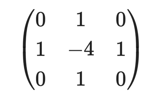
3x3 discrete Laplacian kernel

The center weight is -4 and the four direct neighbors each get +1. When you apply this kernel to a pixel, you're computing the difference between that pixel's intensity and the average of its four neighbors - the discrete version of the same "how does this point compare to its surroundings" question from before.

Practical considerations

Raw Laplacian filtering is sensitive to noise. A single noisy pixel produces a sharp intensity spike, and the Laplacian will flag it as an edge.

The standard fix is to smooth the image first with a Gaussian blur, then apply the Laplacian. This combination is called the Laplacian of Gaussian (LoG). The Gaussian suppresses noise, and the Laplacian finds the real edges.

In deep learning, convolutional neural networks learn their own edge-detection filters from data - but those learned filters often resemble the Laplacian kernel. So in a way, the math that made the Laplacian useful in classical computer vision is the same math neural networks rediscover on their own.

Discrete vs. Continuous Laplacian

The Laplacian is three related ideas that show up in different contexts.

Understanding which version you're working with saves a lot of confusion when you move between calculus textbooks, numerical code, and graph ML papers.

The continuous Laplacian

The continuous Laplacian is the one from calculus. For a smooth function f defined over a continuous space, it's the sum of second partial derivatives:

The continuous Laplacian

This version assumes your function is smooth and differentiable everywhere. It's the theoretical foundation - but real data is never continuous. You can't compute exact derivatives on a grid of pixels or a table of measurements.

The discrete Laplacian

When you move from continuous functions to sampled data, derivatives get replaced with finite differences - approximations computed from neighboring values.

For a 1D function sampled at evenly spaced points, the discrete second derivative at point i is:

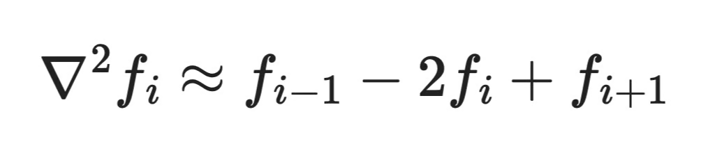
The discrete Laplacian

You're comparing the value at i to its two neighbors. The same idea extends to 2D grids (images), 3D volumes, and beyond. The convolution kernels from the image processing section are exactly this - finite difference approximations of the continuous Laplacian, applied to a pixel grid.

This discretization makes the Laplacian computable in numerical methods and ML pipelines. Any time you apply a Laplacian filter in code, you're running a finite difference approximation, not the exact calculus operator.

The graph Laplacian

The graph Laplacian takes discretization one step further. Instead of a regular grid with uniform spacing, you have an arbitrary set of nodes connected by edges with varying weights.

There's no notion of "neighboring pixel" here - just nodes and the connections between them. The graph Laplacian L = D - A replaces the finite difference structure with adjacency structure. The same core question remains: how does a node's value compare to its neighbors? But "neighbors" is now defined by the graph, not by spatial proximity.

Why this matters in ML

Most ML data doesn't live on a regular grid. Molecules, social networks, knowledge graphs, and 3D point clouds all have irregular structure. You can't apply a standard finite difference Laplacian to them.

The graph Laplacian solves this by making the neighborhood structure explicit through the adjacency matrix. It's why graph neural networks and spectral methods can apply Laplacian-based operations to data that has no natural coordinate system.

Worked Example: Computing a Laplacian

Let's make this concrete with two examples - one continuous, one graph-based.

Example 1: Continuous Laplacian of f(x, y) = x² + y²

Take the function f(x, y) = x² + y². This is a simple paraboloid - a bowl shape that curves upward in every direction.

To compute the Laplacian, you need the second partial derivative with respect to each variable.

First, with respect to x:

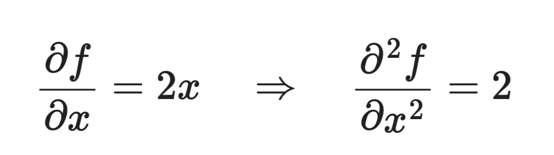
Continuous Laplacian computation (1)

Then with respect to y:

Continuous Laplacian computation (2)

And now just sum them:

Continuous Laplacian computation (3)

The Laplacian is a constant 4 everywhere. That makes sense since a paraboloid has the same curvature at every point. The positive value tells you the function curves upward in all directions, consistent with the bowl shape.

Example 2: Graph Laplacian for a small graph

Take a graph with 4 nodes and the following edges:

• Node 1 connects to nodes 2 and 3
• Node 2 connects to nodes 1 and 4
• Node 3 connects to node 1
• Node 4 connects to node 2

The adjacency matrix A encodes the connections:

Graph Laplacian computation (1)

The degree matrix D puts each node's connection count on the diagonal:

Graph Laplacian computation (2)

Nodes 1 and 2 each have 2 connections. Nodes 3 and 4 each have 1.

Finally, subtract to get L = D - A:

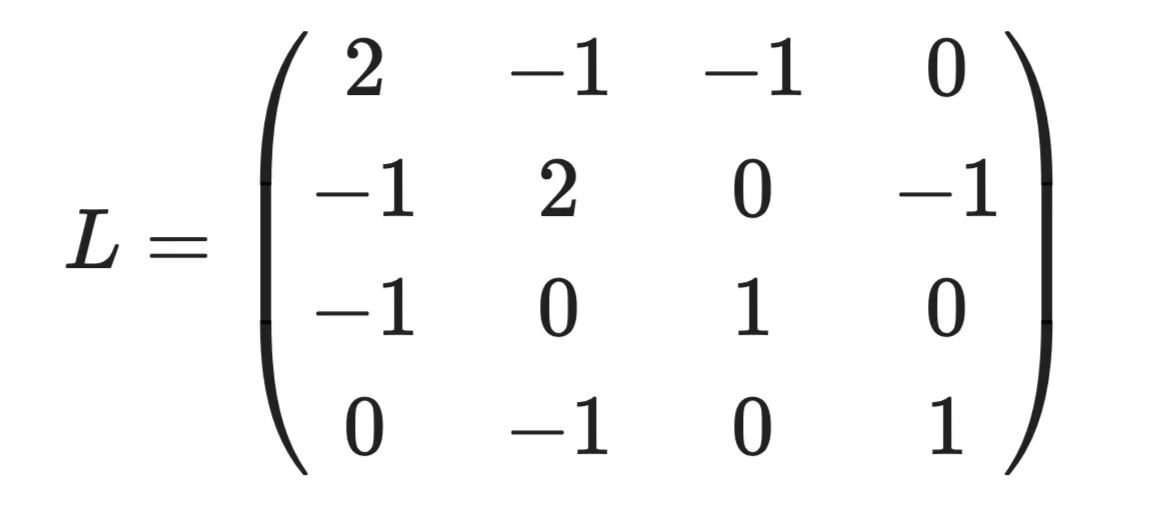
Graph Laplacian computation (3)

Here's how to read this matrix: Row 1 says: node 1 has degree 2, and it's connected to nodes 2 and 3 (the -1 entries). Row 3 says: node 3 has degree 1, connected only to node 1. The zeros tell you which pairs of nodes share no edge.

You can also compute it in Python to verify:

import numpy as np

A = np.array([
    [0, 1, 1, 0],
    [1, 0, 0, 1],
    [1, 0, 0, 0],
    [0, 1, 0, 0]
])

D = np.diag(A.sum(axis=1))
L = D - A

print(L)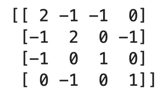

Graph Laplacian computation in Python

Common Confusions

The Laplacian is similar to few other concepts, and the differences aren't always obvious from the names alone. In this section, I’ll try to eliminate all points of confusion.

Laplacian vs. gradient

The gradient ∇f is a vector. It points in the direction of steepest increase and its magnitude tells you how fast the function is rising. It uses first derivatives.

The Laplacian ∇²f is a scalar. It doesn't tell you which direction to move - it tells you about the shape of the function at a point. It's built from second derivatives.

Laplacian vs. Hessian

This one trips people up most often.

The Hessian H is a matrix of all second partial derivatives. For a function with n inputs, it's an n × n matrix that captures how the gradient changes along every pair of axes. It gives you the full curvature picture.

The Laplacian is the trace of the Hessian - the sum of its diagonal entries. You lose the off-diagonal curvature information, but you get a single number that's fast to compute.

Use the Hessian when you need the complete curvature breakdown. Use the Laplacian when a scalar summary is enough.

Graph Laplacian vs. differential operator

These share a name and the same core intuition, but they operate on completely different objects.

The differential Laplacian acts on smooth, continuous functions. It requires derivatives, which means it assumes your function is differentiable everywhere.

The graph Laplacian L = D - A acts on graphs - discrete structures with nodes and edges. There are no derivatives involved. It measures how a value at each node differs from its neighbors using matrix operations.

The connection is conceptual, not computational. Both measure local deviation from a neighborhood average, but are entirely different.

Sign conventions

Some fields define the Laplacian with a negative sign: -∇²f. You'll see this in physics and in some ML papers on graph neural networks. The negative Laplacian −L is positive semi-definite, which has nicer properties for certain optimization problems and makes eigenvalue analysis cleaner.

When you read a paper and the Laplacian's eigenvalues are all non-negative, check whether they're using L or -L. The math is equivalent, but mixing conventions could lead you to wrong results.

Why the Laplacian Matters in Data Science

At this point, you've seen the Laplacian show up across calculus, graph theory, image processing, and optimization. The same operator is solving the same fundamental problem in different contexts: measuring how a value at one point relates to its surroundings.

Here's where that shows up in data science:

• Graph-based ML: The graph Laplacian L = D - A is the foundation of spectral methods. Any time your data has a natural graph structure, the Laplacian gives you a matrix that encodes the full connectivity pattern in a form you can do linear algebra on

• Clustering: Spectral clustering uses the eigenvectors of L to find groups that pure distance-based methods miss. It works well when clusters aren't convex or linearly separable

• Semi-supervised learning: Many semi-supervised methods use the graph Laplacian to propagate labels from labeled to unlabeled nodes. The assumption is that connected nodes likely share the same label, and the Laplacian quantifies how smoothly labels should vary across the graph

• Manifold learning: Algorithms like Laplacian Eigenmaps use the graph Laplacian to find low-dimensional representations of high-dimensional data. The eigenvectors of L map nearby points in the original space to nearby points in the reduced space

• Image feature extraction: The discrete Laplacian detects edges and regions of rapid intensity change. Those features feed directly into both classical computer vision pipelines and as priors in deep learning architectures

To sum it up, the Laplacian is one of the few mathematical tools that scales from a single calculus equation all the way up to large graph neural networks.

Conclusion

The Laplacian starts as a calculus operator, a way to measure curvature in continuous functions. By the time you reach graph-based ML, it's a matrix that encodes the structure of an entire network. The core idea is exactly the same, only the form is different.

Enroll in our Linear Algebra for Data Science in R course to get hands-on experience with many concepts and topics covered by this article.