Ensemble Learning in Python: A Hands-On Guide to Random Forest and XGBoost

A single decision tree is easy to interpret but tends to overfit. A simple linear model generalizes well but misses complex patterns. Each model type has blind spots that limit its accuracy on real-world data.

Ensemble methods address this by combining multiple models into a single model. Instead of relying on a single predictor, they aggregate predictions from many models so that individual errors cancel out. The result is usually more accurate than any single model alone.

In this tutorial, I’ll teach you the differences between core ensemble methods and focus on the two most popular ensemble algorithms: Random Forest and XGBoost. 

You'll learn how each one works, implement both on a multiclass classification problem, and compare their performance. The goal is to give you a practical understanding of when to use each approach and how to tune them for your own projects.

If you’re looking for some further hands-on practice, I recommend checking out the Ensemble Methods in Python course. 

What Is Ensemble Learning?

Ensemble learning trains multiple models and combines their predictions into a single output. The idea is simple: different models make different mistakes, so averaging or voting across many models tends to cancel out individual errors.

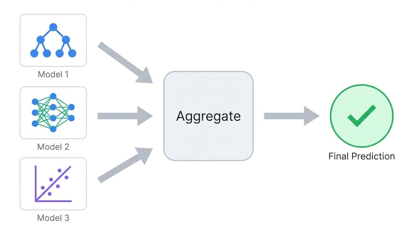
Ensemble learning combines predictions from multiple models into a single aggregated output

Consider a classification task where you train five decision trees. Each tree might get 80% of predictions right, but they won't all fail on the same examples. When you aggregate their votes, the majority often gets it right even when one or two trees are wrong. This is the core principle behind all ensemble methods.

The models inside an ensemble are called base learners. They can be any algorithm, but decision trees are the most common choice because they're fast to train and naturally produce diverse predictions when given different data subsets.

The bias-variance trade-off

Model errors come from two sources: bias and variance.

Bias is the error from oversimplifying the problem. A linear model trying to fit a curved relationship has high bias because it can't represent the true pattern, no matter how much data you give it. High-bias models produce similar predictions across different training sets, but those predictions are always off-target.

Variance is the error from being too sensitive to training data. A deep decision tree that memorizes the training set has high variance because it captures noise along with signal. If you retrained the same tree on a slightly different sample, you'd get wildly different predictions. The model fits the training data well, but falls apart on anything new.

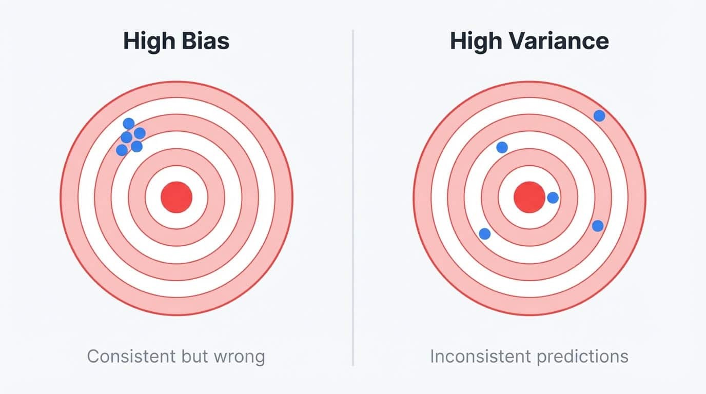
Bias vs variance illustrated with dartboards: high bias shows consistent but off-target predictions, high variance shows scattered inconsistent predictions

You can think of it as a stability problem. High-bias models are stable but wrong in the same way every time. High-variance models are unstable and wrong in different ways depending on what data they happened to see. 

The ideal model is both stable and accurate, but reducing one type of error often increases the other.

Decision trees sit squarely in the high-variance camp. They use greedy splitting, meaning small changes in the training data can produce completely different tree structures. 

Train the same tree algorithm on two random samples from the same population, and you might get two models that look nothing alike. This instability makes individual trees unreliable, but it also makes them perfect building blocks for ensembles. 

High variance means there's room for improvement through aggregation. Trees are also fast to train and handle non-linear relationships without manual feature engineering, which is why Random Forest and XGBoost both use them despite attacking different parts of the bias-variance problem.

Ensemble methods break this trade-off by combining multiple models:

Bagging 

Bagging trains many models in parallel on random subsets of data, then averages their predictions. This reduces variance by smoothing out the quirks of individual models. The intuition is straightforward: if each model makes somewhat independent errors, averaging tends to cancel those errors out. The more models you combine, the more stable the final prediction becomes. This is why Random Forest defaults to 100 trees rather than 10.

Boosting 

Boosting trains models sequentially, where each new model focuses on the mistakes of the previous ones. This reduces bias by building a strong learner from many weak ones.

Ensemble Learning: Bagging vs Boosting

Let’s break down how bagging and boosting work in practice.

Bagging: parallel training to reduce variance

Bagging stands for bootstrap aggregating. The process has three steps:

1.      Create multiple training sets by sampling from the original data with replacement (bootstrap samples)

2.     Train one model on each bootstrap sample independently

3.     Combine predictions by averaging (regression) or majority vote (classification)

Bootstrap sampling means each training set is the same size as the original, but some examples appear multiple times while others are left out entirely. On average, each bootstrap sample contains about 63% of the unique examples from the original data. The remaining 37% are called out-of-bag samples and can be used for validation.

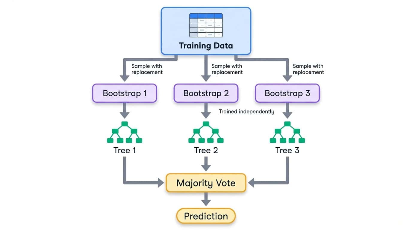
Bagging workflow showing training data split into bootstrap samples, each training an independent decision tree, then combining via majority vote

Because each model sees a different slice of the data, they develop different quirks. Some overfit to one region of the feature space, others to a different region. When you aggregate their predictions, these individual errors tend to wash out. The ensemble prediction is more stable than any single model.

Training happens in parallel since the models don't depend on each other. This makes bagging straightforward to scale across multiple CPU cores. Random Forest, which you'll implement later in this tutorial, is the most widely used bagging algorithm. For a deeper look at the theory, see DataCamp's guide to bagging in machine learning.

Boosting: sequential training to reduce bias

Boosting takes a different approach. Instead of training models independently, it trains them one after another, with each new model focusing on examples the previous models got wrong.

The general process looks like this:

1.     Train a weak model on the full training set

2.     Identify which examples the model predicted poorly

3.     Train the next model with extra emphasis on those hard examples

4.     Repeat, adding models that correct the remaining errors

5.     Combine all models into a weighted sum, where better-performing models get higher weights

The term "weak learner" means a model that performs only slightly better than random guessing. Decision stumps (trees with a single split) are a common choice. Individually, a stump is nearly useless. But boosting stacks hundreds of them, each one chipping away at the errors left by the previous ones. The final ensemble is a strong learner built from many weak contributions.

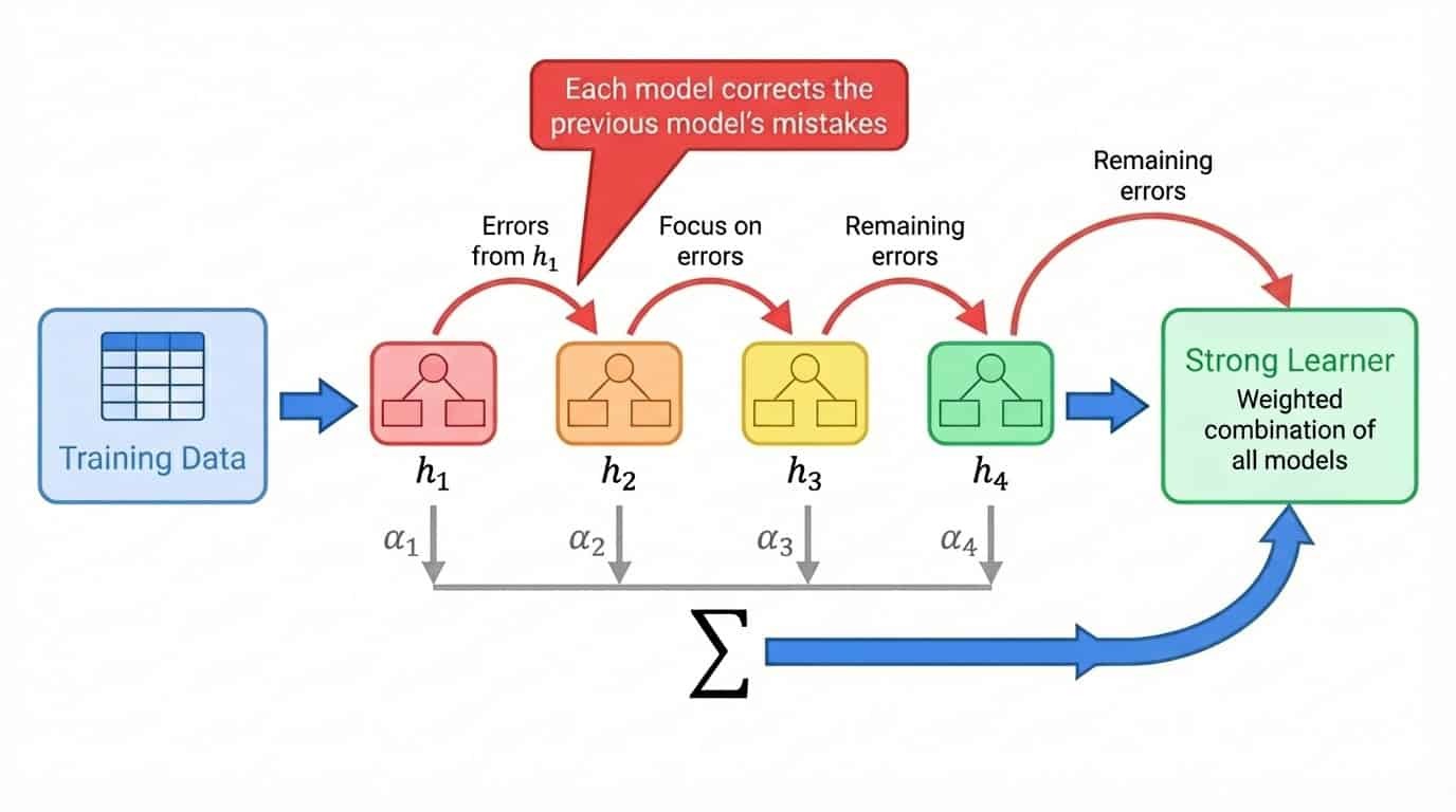
Boosting workflow showing sequential model training where each model corrects the previous model's errors, combined into a weighted sum

Unlike bagging, boosting is inherently sequential. You can't train model 47 until you know which examples models 1 through 46 struggled with. This makes boosting slower to train, but it often produces higher accuracy because each model is purpose-built to fix specific weaknesses in the ensemble.

XGBoost, which you'll implement later in this tutorial, is a gradient boosting algorithm that has become the go-to choice for tabular data. I recommend the introduction to boosting guide, which covers the math in more detail if you want to dig deeper.

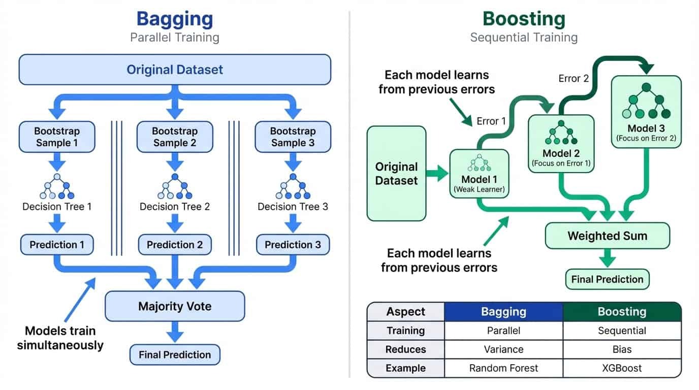
Side-by-side comparison of bagging and boosting: bagging uses parallel training to reduce variance, boosting uses sequential training to reduce bias

Other Ensemble Learning Approaches

Bagging and boosting are the most widely used ensemble strategies, but they're not the only options. Before diving into Random Forest and XGBoost, it's worth knowing what else exists.

Voting and averaging

The simplest way to combine models is to let them vote. In hard voting, each model makes a prediction, and the class with the most votes wins. If you have a logistic regression, a support vector machine, and a decision tree, and two of them predict class A while one predicts class B, the ensemble outputs class A.

Soft voting takes this further by averaging the predicted probabilities instead of counting discrete votes. A model that predicts class A with 90% confidence contributes more to the final decision than one that predicts A with 51% confidence. This usually outperforms hard voting because it captures how certain each model is.

You can also assign weights to give stronger models more influence. If your logistic regression reliably outperforms the others on validation data, you might weight its predictions at 2x while keeping the others at 1x.

Voting works best when combining models that approach the problem differently. A linear model, a tree-based model, and a nearest-neighbor model each have different blind spots. Their combined prediction often beats any individual, even if no single model is very strong. scikit-learn provides VotingClassifier and VotingRegressor for this purpose.

Stacking and blending

Stacking takes the ensemble idea one level deeper. Instead of averaging predictions, you train a second model (called a meta-learner) to combine them. The process works like this: train several base models, collect their predictions on a validation set, then train the meta-learner to map those predictions to the correct labels. The meta-learner learns which base model to trust in which situations.

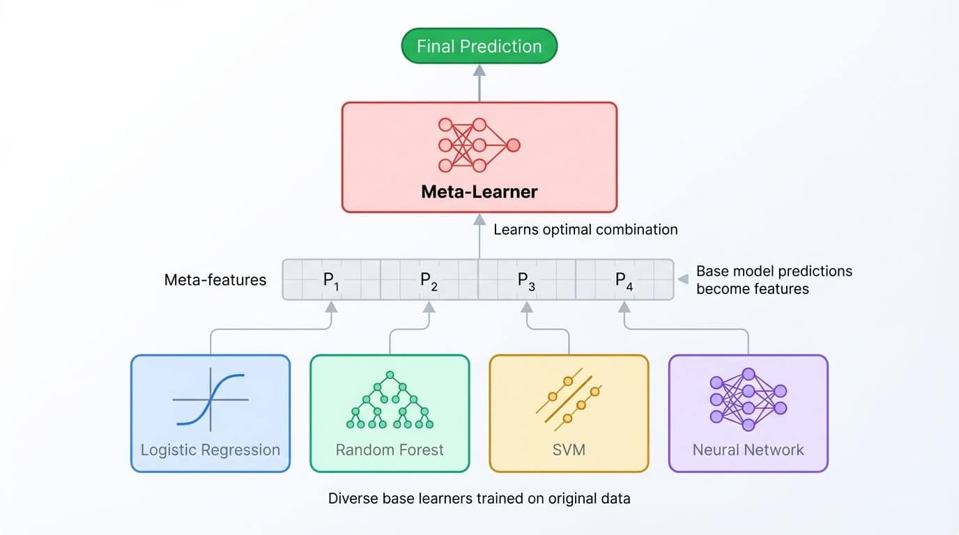
Stacking ensemble architecture showing diverse base models feeding predictions to a meta-learner that combines them for the final output

Blending is a simpler variant that uses a single holdout set rather than cross-validation folds. It's faster to implement but wastes some training data and can be more prone to overfitting the holdout set.

Both techniques can squeeze out extra accuracy, but the gains are often small (0.1-0.5% improvement) relative to the added complexity. Stacked ensembles are harder to debug, slower to train, and more difficult to explain to stakeholders. They shine in Kaggle competitions where every decimal point matters and training time is unlimited, but they're rarely worth the overhead in production.

Interestingly, most stacked ensembles use Random Forest and XGBoost as base learners anyway. These two algorithms are so strong that stacking often just becomes an elaborate way to average their predictions.

Why this tutorial focuses on bagging and boosting

This tutorial sticks to Random Forest (bagging) and XGBoost (boosting) because they handle the vast majority of real-world tabular data problems. They're simpler to implement, easier to tune, and more straightforward to maintain than multi-level stacked ensembles.

If you want to go deeper into voting and stacking, DataCamp's Ensemble Methods in Python course covers the full range of techniques. For now, let's get hands-on with the dataset.

Setting Up Data for Ensemble Classification

This tutorial uses the Dry Beans dataset from the UCI Machine Learning Repository. Researchers Koklu and Ozkan (2020) photographed 13,611 dry beans from seven varieties and extracted 16 geometric features from each image, including area, perimeter, axis lengths, and shape factors. The task is to classify each bean by variety based on these measurements.

The dataset works well for this tutorial because it's a clean multiclass problem with all numeric features. No missing values, no categorical encoding, no text preprocessing. You can focus entirely on the ensemble methods.

Loading and splitting the data

!uv add ucimlrepo scikit-learn pandas xgboost

 from ucimlrepo import fetch_ucirepo
 from sklearn.model_selection import train_test_split
 import pandas as pd

 dry_bean = fetch_ucirepo(id=602)
 X = dry_bean.data.features
 y = dry_bean.data.targets.values.ravel()

 print(f"Features shape: {X.shape}")
 print(f"Target classes: {pd.Series(y).nunique()}")

Features shape: (13611, 16)
 Target classes: 7

X.head()

pd.Series(y).value_counts()

DERMASON	3546
 SIRA    	2636
 SEKER   	2027
 HOROZ   	1928
 CALI    	1630
 BARBUNYA	1322
 BOMBAY   	522

The classes are reasonably balanced, with Dermason being the most common and Bombay the least. A stratified split preserves these proportions in both training and test sets:

X_train, X_test, y_train, y_test = train_test_split(
 	X, y, test_size=0.2, random_state=42, stratify=y
 )
 print(f"Training set: {X_train.shape[0]} samples")
 print(f"Test set: {X_test.shape[0]} samples")

Training set: 10888 samples
 Test set: 2723 samples

Random Forest Classifier in Python

With the data ready, it's time to train the first ensemble model. This section covers how Random Forest works under the hood, walks through training and evaluation, and shows how to tune its hyperparameters.

How Random Forest works

Random Forest applies bagging to decision trees with one additional twist. Each tree is trained on a bootstrap sample of the data (as covered in the previous section), but at each split, the algorithm only considers a random subset of features rather than all of them.

This feature randomization prevents trees from becoming too similar. Without it, the same strong predictors would dominate every tree, and the ensemble would just be many copies of nearly identical models. 

By forcing each split to choose among a limited feature set, the algorithm creates diverse trees that make different errors. When these trees vote together, their individual mistakes tend to cancel out.

For classification, scikit-learn defaults to considering the square root of the total features at each split. With 16 features in the Dry Beans dataset, each split evaluates only 4 randomly chosen features. The result is an ensemble of decorrelated trees that generalizes better than any single tree could.

Training and evaluation

from sklearn.ensemble import RandomForestClassifier
 from sklearn.metrics import classification_report, accuracy_score

 rf = RandomForestClassifier(n_estimators=100, random_state=42)
 rf.fit(X_train, y_train)
 y_pred_rf = rf.predict(X_test)

 print(f"Accuracy: {accuracy_score(y_test, y_pred_rf):.4f}")
 print(classification_report(y_test, y_pred_rf))

Accuracy: 0.9199
           	precision	recall  f1-score   support

 	BARBUNYA   	0.94      0.89  	0.92   	265
   	BOMBAY   	1.00      1.00  	1.00   	104
     	CALI   	0.94      0.94  	0.94   	326
 	DERMASON   	0.90      0.92  	0.91   	709
    	HOROZ   	0.96      0.95  	0.96   	386
    	SEKER   	0.94      0.96  	0.95   	406
     	SIRA   	0.86      0.85  	0.86   	527

 	accuracy                       	0.92 	 2723
    macro avg   	0.93      0.93  	0.93  	2723
 weighted avg   	0.92  	0.92      0.92  	2723

This code creates a forest of 100 decision trees, trains them on the bootstrap samples, and generates predictions by majority vote. The random_state parameter fixes the random seed so results are reproducible.

The classification report breaks down performance by class. Precision measures how many predicted positives were correct, recall measures how many actual positives were found, and F1-score is their harmonic mean. Bombay beans are classified perfectly (likely because they're physically distinct), while Sira beans are the hardest to distinguish from other varieties.

One advantage of Random Forest is interpretable feature importances. The algorithm tracks how much each feature reduces impurity (the Gini index, by default) across all trees, giving you a built-in measure of which variables matter most:

import matplotlib.pyplot as plt

 importances = rf.feature_importances_
 feature_names = X.columns
 sorted_idx = importances.argsort()[::-1][:10]

 plt.figure(figsize=(10, 6))
 plt.barh(range(10), importances[sorted_idx][::-1])
 plt.yticks(range(10), feature_names[sorted_idx][::-1])
 plt.xlabel("Feature importance")
 plt.title("Top 10 features (Random Forest)")
 plt.tight_layout()
 plt.show()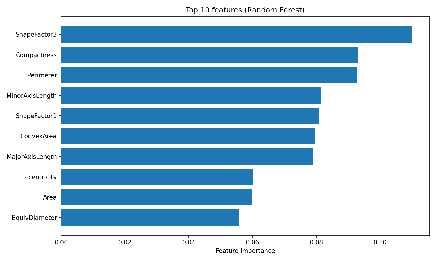

Random Forest feature importance

The feature_importances_ attribute returns an array of scores summing to 1, where higher values indicate features that contributed more to splitting decisions. ShapeFactor3 and Compactness contribute the most to classification, followed by geometric measurements like Perimeter and MinorAxisLength. These shape-based features capture the visual differences between bean varieties that the original researchers designed the dataset to measure.

Hyperparameters worth tuning

Random Forest has three main hyperparameters worth tuning:

• n_estimators: The number of trees in the forest. More trees produce more stable predictions but take longer to train. Returns diminish past 200 trees for most datasets.
• max_depth: The maximum depth of each tree. The default (None) grows trees until leaves are pure or contain fewer than 2 samples. Lower values can prevent overfitting.
• max_features: The number of features considered at each split. The default "sqrt" works well for classification. Using "log2" increases diversity at the cost of individual tree accuracy.

A quick grid search over these parameters:

from sklearn.model_selection import GridSearchCV

 param_grid = {
 	"n_estimators": [100, 200],
 	"max_depth": [10, 20, None],
 	"max_features": ["sqrt", "log2"]
 }

 grid_search = GridSearchCV(
     RandomForestClassifier(random_state=42),
 	param_grid,
 	cv=3,
 	scoring="accuracy",
 	n_jobs=-1
 )
 grid_search.fit(X_train, y_train)

 print(f"Best params: {grid_search.best_params_}")
 print(f"Best CV accuracy: {grid_search.best_score_:.4f}")

Best params: {'max_depth': None, 'max_features': 'sqrt', 'n_estimators': 200}
 Best CV accuracy: 0.9244

GridSearchCV tries every combination of parameters in the grid and evaluates each one using cross-validation. The cv=3 argument splits the training data into 3 folds, training on 2 and validating on 1, rotating through all combinations. The n_jobs=-1 flag parallelizes the search across all available CPU cores.

y_pred_tuned = grid_search.best_estimator_.predict(X_test)
 print(f"Tuned test accuracy: {accuracy_score(y_test, y_pred_tuned):.4f}")

Tuned test accuracy: 0.9214

Tuning bumps accuracy from 92.0% to 92.1%, a modest improvement. The best configuration uses the defaults for max_depth and max_features, with 200 trees instead of 100. Random Forest often performs well out of the box, which is one of its main appeals. For a deeper look at Random Forest and its parameters, see DataCamp's Random Forest classification tutorial.

XGBoost Classifier in Python

XGBoost (Extreme Gradient Boosting) takes a different path to accuracy than Random Forest. Where Random Forest reduces variance by averaging independent trees, XGBoost reduces bias by training trees sequentially, with each new tree correcting the mistakes of the ensemble so far. This section covers how gradient boosting works, what makes XGBoost special, and how to train and tune it on the Dry Beans dataset.

How gradient boosting works

Gradient boosting builds an ensemble one tree at a time. The first tree makes predictions on the original target. The second tree is trained not on the original target, but on the residual errors from the first tree. The third tree fits the residuals left over after adding the second tree's predictions. This continues for hundreds of rounds, with each new tree chipping away at whatever error remains.

The term "gradient" refers to how the algorithm decides what to fit. At each step, it computes the gradient of the loss function with respect to the current predictions. For regression with squared error loss, this gradient is just the residual (actual minus predicted). For classification, the math is more involved, but the intuition is the same: each tree is trained to move predictions in the direction that reduces loss the most.

A learning rate parameter shrinks each tree's contribution before adding it to the ensemble. With a learning rate of 0.1, for example, only 10% of each tree's prediction is added. This forces the algorithm to take smaller steps and typically improves generalization. The trade-off is that you need more trees to reach the same level of fit. Small learning rate plus many trees tends to produce better results than large learning rate with few trees.

What makes XGBoost different

XGBoost is one of several gradient boosting implementations, alongside LightGBM and CatBoost. It became popular because it added several improvements over earlier implementations like scikit-learn's GradientBoostingClassifier.

The main additions are:

• L1 and L2 regularization built into the objective function, which penalizes complex trees and reduces overfitting
•  Native handling of missing values by learning the optimal direction for missing data at each split
• Parallelized tree construction within each boosting round, making it faster than purely sequential implementations
• Column subsampling, which randomly samples features at each tree or split (similar to Random Forest's feature randomization)

These features make XGBoost both faster and more resistant to overfitting than vanilla gradient boosting. The regularization parameters give you direct control over model complexity, which is useful when working with noisy or high-dimensional data.

Training and evaluation

XGBoost expects numeric class labels rather than strings, so the first step is encoding the target variable:

from xgboost import XGBClassifier
 from sklearn.preprocessing import LabelEncoder

 le = LabelEncoder()
 y_train_encoded = le.fit_transform(y_train)
 y_test_encoded = le.transform(y_test)

 xgb = XGBClassifier(n_estimators=100, random_state=42, eval_metric="mlogloss")
 xgb.fit(X_train, y_train_encoded)
 y_pred_xgb = xgb.predict(X_test)

 print(f"Accuracy: {accuracy_score(y_test_encoded, y_pred_xgb):.4f}")
 print(classification_report(y_test_encoded, y_pred_xgb, target_names=le.classes_))

Accuracy: 0.9232
           	precision	recall  f1-score   support

 	BARBUNYA   	0.95      0.89  	0.92   	265
   	BOMBAY   	1.00      1.00  	1.00   	104
     	CALI   	0.94      0.94  	0.94   	326
 	DERMASON   	0.90      0.93  	0.91   	709
    	HOROZ   	0.96      0.96  	0.96   	386
    	SEKER   	0.95      0.96  	0.95   	406
     	SIRA   	0.87      0.86  	0.87   	527

 	accuracy                       	0.92 	 2723
    macro avg   	0.94      0.93  	0.93  	2723
 weighted avg   	0.92  	0.92      0.92  	2723

The LabelEncoder maps class names to integers (0 through 6) and stores the mapping so you can convert predictions back to class names. The eval_metric="mlogloss" argument tells XGBoost to use multiclass log loss for internal evaluation.

Out of the box, XGBoost achieves 92.3% accuracy, slightly higher than Random Forest's 92.0%. The per-class pattern is similar: Bombay beans are classified perfectly, while Sira beans remain the hardest to distinguish.

XGBoost provides feature importances based on gain, which measures the average improvement in accuracy each feature contributes across all splits where it's used:

importances_xgb = xgb.feature_importances_
 sorted_idx_xgb = importances_xgb.argsort()[::-1][:10]

 plt.figure(figsize=(10, 6))
 plt.barh(range(10), importances_xgb[sorted_idx_xgb][::-1])
 plt.yticks(range(10), feature_names[sorted_idx_xgb][::-1])
 plt.xlabel("Feature importance (gain)")
 plt.title("Top 10 features (XGBoost)")
 plt.tight_layout()
 plt.show()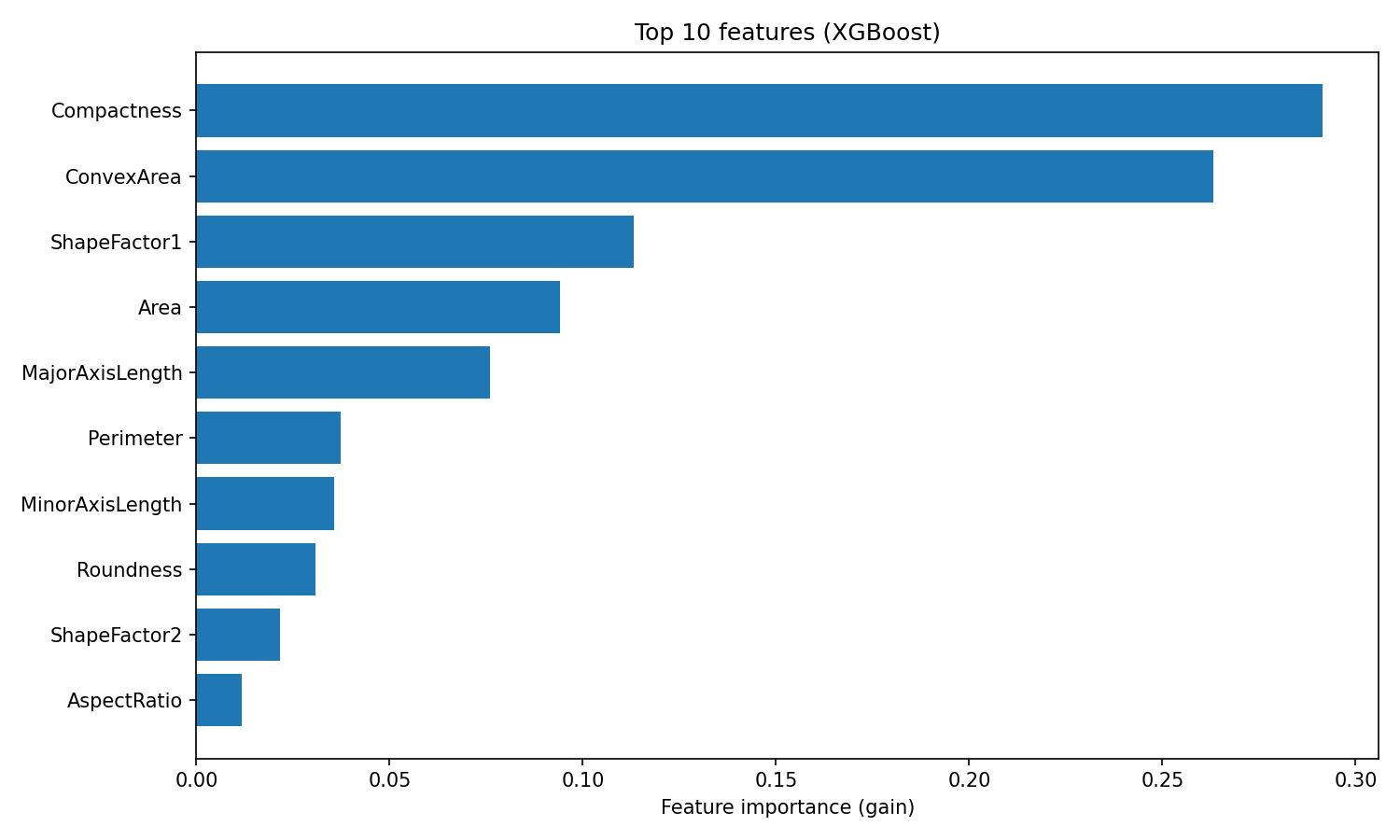

XGBoost feature importance

The ranking differs from Random Forest. XGBoost puts Compactness and ConvexArea at the top, while Random Forest ranked ShapeFactor3 first. 

This difference reflects how the two algorithms use features: Random Forest measures how often a feature reduces impurity across many independent trees, while XGBoost measures how much accuracy each feature adds when correcting residuals. Both rankings are valid, they just capture different aspects of feature usefulness.

Hyperparameters worth tuning

XGBoost has more tuning knobs than Random Forest, reflecting its greater flexibility. The main parameters to consider are:

• learning_rate: Shrinkage applied to each tree (default 0.3). Lower values require more trees but often generalize better.
• max_depth: Maximum tree depth (default 6). Shallower trees reduce overfitting. XGBoost's default is more conservative than Random Forest's unlimited depth.
• n_estimators: Number of boosting rounds. More rounds allow finer corrections, especially with a low learning rate.
• reg_alpha: L1 regularization on leaf weights (default 0). Higher values push weights toward zero, creating sparser models.
• reg_lambda: L2 regularization on leaf weights (default 1). Higher values penalize large weights, smoothing predictions.

A grid search over a few of these parameters:

param_grid_xgb = {
 	"learning_rate": [0.05, 0.1],
 	"max_depth": [4, 6],
 	"n_estimators": [100, 200],
 	"reg_lambda": [1, 5]
 }

 grid_search_xgb = GridSearchCV(
 	XGBClassifier(random_state=42, eval_metric="mlogloss"),
 	param_grid_xgb,
 	cv=3,
 	scoring="accuracy",
 	n_jobs=-1
 )
 grid_search_xgb.fit(X_train, y_train_encoded)

 print(f"Best params: {grid_search_xgb.best_params_}")
 print(f"Best CV accuracy: {grid_search_xgb.best_score_:.4f}")

Best params: {'learning_rate': 0.1, 'max_depth': 4, 'n_estimators': 200, 'reg_lambda': 5}
 Best CV accuracy: 0.9284

y_pred_xgb_tuned = grid_search_xgb.best_estimator_.predict(X_test)
 print(f"Tuned test accuracy: {accuracy_score(y_test_encoded, y_pred_xgb_tuned):.4f}")

Tuned test accuracy: 0.9251

The best configuration uses shallower trees (max_depth=4), more regularization (reg_lambda=5), and twice as many boosting rounds (n_estimators=200). This pattern is common: XGBoost often performs best with weaker individual trees combined through more boosting rounds. Tuning improves test accuracy from 92.3% to 92.5%.

For a deeper look at XGBoost's parameters and advanced features like early stopping, see DataCamp's XGBoost in Python tutorial.

Random Forest vs XGBoost

With both models trained and tuned, here's how they compare on the Dry Beans dataset.

Performance comparison

The accuracy numbers favor XGBoost, but the gap shrinks when you look at macro F1. Both models achieve 0.93, meaning they perform equally well across all seven bean classes rather than just excelling on the majority class.

Per-class performance tells a similar story:

Both models rank classes identically. Bombay beans are the easiest to classify (they're the largest and most physically distinct), while Sira beans are the hardest (their shape overlaps with Dermason and Seker). XGBoost's only per-class advantage is a 1-point F1 improvement on Sira.

The practical difference between these models isn't accuracy. It's how much effort you want to spend tuning. Random Forest performed within 0.4% of XGBoost using default parameters. XGBoost needed a grid search over learning rate, tree depth, and regularization to pull ahead.

When to use each algorithm

A reasonable workflow: start with Random Forest to establish a baseline, then try XGBoost if you need to squeeze out extra performance. The best choice depends on your constraints, not some universal ranking of algorithms.

Conclusion

In this tutorial, I’ve shown how bagging and boosting turn weak models into strong ones. Bagging trains models in parallel and averages out their mistakes. Boosting trains them in sequence, with each one fixing what the last got wrong.

Random Forest and XGBoost are the go-to implementations. On the Dry Beans dataset, both landed around 92% accuracy. XGBoost edged ahead after tuning, but Random Forest got there with almost no configuration. That's the real trade-off: Random Forest is low-maintenance, XGBoost rewards the extra effort.

When you're starting a new problem, fit a Random Forest first. It's a solid baseline that takes minutes to set up. If you need to push accuracy higher and have time to tune, switch to XGBoost.

For more hands-on practice with these algorithms, I recommend DataCamp's Machine Learning with Tree-Based Models course.