Hierarchical Clustering: Concept Overview With Examples

So you’ve just been tasked to analyze a large dataset, and you’re required to provide a deep dive cluster analysis. You’ve come across the term “hierarchical clustering”, but what is it exactly, and how does it work? 

In this article, we will explore the concept of hierarchical clustering and provide real-life examples to help you better understand its applications.

What is Hierarchical Clustering?

Hierarchical clustering is an unsupervised learning algorithm used to group similar data points into clusters. It builds a multilevel hierarchy of clusters by either merging smaller clusters into larger ones (agglomerative) or dividing a large cluster into smaller ones (divisive). This results in a tree-like structure known as a dendrogram.

A dendrogram is a visual representation that illustrates the arrangement of clusters and their relationships with each other. The height of the branches in a dendrogram represents the distance or dissimilarity at which clusters merge. Lower heights indicate clusters joined at smaller distances, thus representing higher similarity.

Why hierarchical clustering matters in machine learning

Hierarchical clustering is particularly useful when the number of clusters is not known beforehand. It allows data analysts and data scientists to visually explore the data's structure through dendrograms. 

This technique is also capable of uncovering nested clusters and is widely used in fields like genomics, customer segmentation, and document organization.

For example, let’s say we have a dataset of customer purchase records. Using hierarchical clustering, we can group customers with similar purchasing patterns into clusters and identify potential market segments for targeted marketing strategies.

Hierarchical vs K-Means clustering

When it comes to clustering tasks, most are undecided on two main methods: Hierarchical clustering or K-means clustering.

But what makes them different? Let’s look at their differences below for a clearer picture.

• K-Means:
• Requires the number of clusters to be defined before running.
• Efficient and scalable for large datasets.
• Assumes clusters are spherical and equally sized.
• Hierarchical Clustering:
• Does not require a predefined number of clusters.
• More interpretable due to dendrograms.
• Slower on large datasets but better for exploring structure.

When comparing the two, some areas make hierarchical clustering a stand-out option.

Here are some areas where hierarchical clustering is good:

• Flexibility in cluster selection using dendrograms.
• Good for small datasets or when a visual hierarchy is needed.
• Handles complex cluster shapes.

However, it can have some downsides, such as:

• Computationally expensive
• Sensitive to noisy data and outliers.

You might ask: When should I use hierarchical clustering?

Hierarchical clustering is an excellent choice in the following applications:

• Exploratory data analysis
• Gene expression pattern analysis
• Market segmentation with moderate-sized datasets

Types of Hierarchical Clustering

Within the technique of hierarchical clustering, you’ll expect several types, with each providing different insights and results. The two main types of hierarchical clustering are agglomerative (bottom-up) and divisive (top-down).

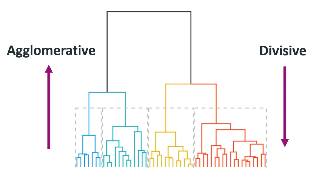
Source: Himanshu Sharma on Medium

1. Agglomerative (Bottom-Up)

Agglomerative clustering starts with each data point as an individual cluster and iteratively merges the closest pair of clusters until only one cluster remains or until a stopping condition is met (like a desired number of clusters).

This method is also called bottom-up because it starts from the bottom (individual data points) and builds up to the top (final cluster).

Step-by-step guide:

1. Treat each data point as a singleton cluster.
2. Compute the pairwise distances between all clusters.
3. Merge the two clusters with the smallest distance.
4. Update the distance matrix to reflect the new set of clusters.
5. Repeat steps 2–4 until all points belong to a single cluster.

This method is widely used due to its simplicity and ease of implementation.

Here’s an example of how this can be implemented in Python:

import numpy as np
from scipy.cluster.hierarchy import linkage, dendrogram, fcluster
import matplotlib.pyplot as plt

# Samples data
data = np.array([[1, 2], [2, 3], [5, 8], [8, 8], [1, 0], [0, 1]])

# Applies agglomerative clustering using Ward's method
Z = linkage(data, method='ward')

# Plots dendrogram
plt.figure(figsize=(8, 4))
dendrogram(Z)
plt.title('Agglomerative Clustering Dendrogram')
plt.xlabel('Data Points')
plt.ylabel('Distance')
plt.show()

# Extracts clusters (e.g., form 2 clusters)
clusters = fcluster(Z, t=2, criterion='maxclust')
print("Cluster assignments:", clusters)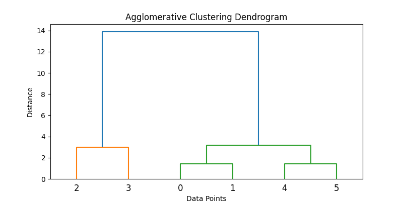

2. Divisive (Top-Down)

Divisive clustering starts with all data points in a single cluster and recursively splits them into smaller clusters. The process continues until each data point is in its own individual cluster.

It is also known as a top-down approach, as it starts at the top (single cluster) and breaks it down into smaller clusters.

Step-by-step guide:

1. Start with one large cluster containing all data points.
2. Split the cluster into two that are as different as possible.
3. Reapply the splitting process recursively to each resulting cluster.

Divisive methods are typically more computationally expensive due to their recursive nature, and accuracy depends greatly on the splitting strategy. Agglomerative methods are more common due to ease of implementation and widespread software support.

Note: Divisive hierarchical clustering is not as readily supported in standard Python libraries as agglomerative clustering. One approach is to use clustering algorithms like k-means recursively.

Here’s a code concept of a simulated recursive k-means splitting:

from sklearn.cluster import KMeans

def divisive_clustering(data, depth=2):
    if depth == 0 or len(data) <= 1:
        return [data]

    kmeans = KMeans(n_clusters=2, random_state=42).fit(data)
    labels = kmeans.labels_
    cluster1 = data[labels == 0]
    cluster2 = data[labels == 1]

    return divisive_clustering(cluster1, depth - 1) + divisive_clustering(cluster2, depth - 1)

# Run recursive splitting to simulate divisive clustering
split_clusters = divisive_clustering(data, depth=2)
for i, cluster in enumerate(split_clusters):
    print(f"Cluster {i+1} size: {len(cluster)}")

This simplified code illustrates a conceptual approach to divisive clustering using recursive K-means. Note, however, that standard divisive methods like DIANA use different splitting criteria.

Key Concepts and Terminologies

Hierarchical clustering involves some key concepts and terminologies that are important to understand. To fully grasp the process, we will go over these concepts in more detail below.

1. Dendrograms

A dendrogram is a tree-like structure that visualizes the process of hierarchical clustering. Each level of the tree represents a merge or split operation, and the height of the branches represents the distance (or dissimilarity) at which clusters were joined.

Here’s why it's important:

• Allows visual inspection of clusters at different levels.
• By "cutting" the dendrogram at a certain height, you can choose the number of clusters that best fits the data.

2. Linkage criteria

Linkage criteria determine how distances between clusters are calculated during the merging process.

Here are some types of linkage criteria:

Single linkage (minimum)

This criterion looks at the distance between the closest points of two clusters. This can result in elongated, chain-like clusters.

from scipy.spatial.distance import pdist, squareform
data = np.array([[1, 2], [2, 3], [5, 8]])
distance_matrix = squareform(pdist(data, metric='euclidean')) 
single_linkage_min = np.min(distance_matrix[0, 1:])
print("Single Linkage Distance between Cluster A (point 1) and Cluster B (point 2, 3):", single_linkage_min)

Complete linkage (maximum)

This criterion looks at the distance between the farthest points of two clusters. This tends to produce compact, evenly sized clusters.

single_linkage_max = np.max(distance_matrix[0, 1:])
print("Complete Linkage Distance between Cluster A and B:", single_linkage_max)

Average linkage (mean)

This criterion looks at the average distance between all points in one cluster to all points in another. This gives a balance between single and complete linkage.

average_linkage = np.mean(distance_matrix[0, 1:])
print("Average Linkage Distance between Cluster A and B:", average_linkage)

These simplified examples illustrate how distances are initially computed. However, during clustering, these criteria (single, complete, average linkage) apply distances iteratively between entire clusters, not just individual points.

Ward's method

Ward’s method is a variation of the average linkage approach that minimizes the sum of squared differences within all clusters. It tends to produce more evenly sized clusters compared to other methods. It also often results in well-separated, spherical clusters.

from scipy.cluster.hierarchy import linkage
linkage_ward = linkage(data, method='ward')
print("Ward's Linkage Matrix:\n", linkage_ward)

Each method has its own strengths and should be chosen based on the data and use case.

3. Distance metrics

The distance metric used influences the clustering result significantly.

Euclidean distance

The Euclidean distance is the straight-line distance between two points in multidimensional space. It is the most commonly used distance metric, especially for geometrically distributed data.

Manhattan distance

Manhattan distance, also known as taxicab or L1 distance, is the sum of absolute differences across dimensions. It is useful for grid-like data such as city blocks or financial transactions.

Cosine similarity

Cosine similarity measures the cosine of the angle between two non-zero vectors. This metric is ideal for text data or when magnitude doesn't matter (e.g., word frequency vectors).

Implementing Hierarchical Clustering in Python

In this section, we'll walk through a practical implementation of agglomerative hierarchical clustering using Python. We'll cover everything from data preprocessing to visualizing results using a dendrogram.

Libraries

We begin by importing the necessary libraries:

import numpy as np
import pandas as pd
from scipy.cluster.hierarchy import dendrogram, linkage, fcluster
from sklearn.preprocessing import StandardScaler
import matplotlib.pyplot as plt

Here’s what we imported in the code above:

• numpy and pandas for data manipulation
• scipy.cluster.hierarchy for clustering and dendrogram generation
• sklearn.preprocessing.StandardScaler for feature scaling
• matplotlib for visualization

Sample data

Before we begin our analysis, let’s create a toy dataset of 2D points and scale it. Scaling is crucial for distance-based algorithms.

This is what our sample dataset would look like.

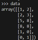
data = np.array([[1, 2], [2, 3], [5, 8], [8, 8], [1, 0], [0, 1]])
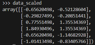
scaler = StandardScaler()
data_scaled = scaler.fit_transform(data)

Here is what the array of data is like after it has been scaled.

Generating a linkage matrix & dendrogram

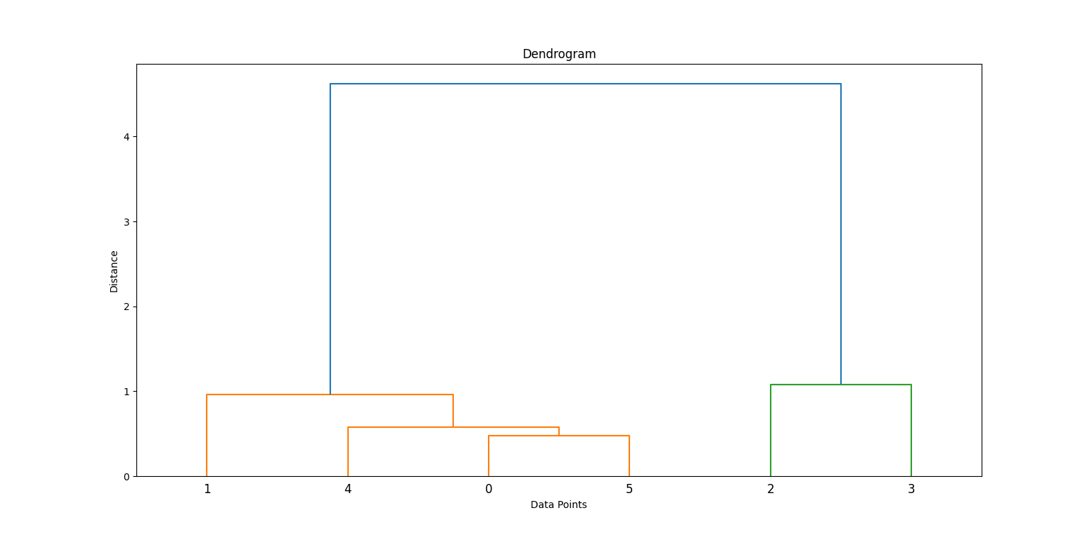
We apply Ward’s method to generate a linkage matrix, which contains hierarchical clustering information. Then, we plot a dendrogram.

linkage_matrix = linkage(data_scaled, method='ward')
plt.figure(figsize=(8, 4))
dendrogram(linkage_matrix)
plt.title('Dendrogram')
plt.xlabel('Data Points')
plt.ylabel('Distance')
plt.show()

In the code above, linkage builds the cluster hierarchy, and dendrogram helps visualize how clusters were formed.

By examining where the vertical lines are longest before a merge, we can decide where to "cut" to form clusters. Look for the highest vertical line that does not intersect with any other clusters. This is where you’ll have to make the cut.

In this case, you’ll need to cut at 2 clusters.

Creating clusters

Next, we cut the dendrogram to get a specific number of clusters using fcluster:

clusters = fcluster(linkage_matrix, t=2, criterion='maxclust')
print(clusters)

plt.scatter(data_scaled[:, 0], data_scaled[:, 1], c=clusters, cmap='rainbow')
plt.title('Clusters')
plt.xlabel('Feature 1')
plt.ylabel('Feature 2')
plt.show()

This assigns each data point to one of two clusters.

Some additional information about the code:

• t=2: Specifies the desired number of clusters.
• criterion='maxclust': Ensures we get exactly t clusters.

You can change t to experiment with different numbers of clusters.

Practical Example: Customer Segmentation

Hierarchical clustering is typically used in customer segmentation. Let’s see how this looks in a practical implementation.

1. Dataset overview

Let’s simulate a dataset representing customers with two features: age and income. We'll use make_blobs to generate this synthetic data.

from sklearn.datasets import make_blobs
X, _ = make_blobs(n_samples=100, centers=3, n_features=2, random_state=42)

2. Preprocessing

Next, we’ll need to standardize the features to normalize scales and improve clustering accuracy.

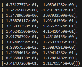
scaler = StandardScaler()
X_scaled = scaler.fit_transform(X)

Here’s what the scaled data looks like:

3. Applying hierarchical clustering

Now that our data has been processed, we’ll plot the dendrogram to visualize how clusters form.

linkage_matrix = linkage(X_scaled, method='ward')
plt.figure(figsize=(10, 5))
dendrogram(linkage_matrix)
plt.title('Customer Dendrogram')
plt.xlabel('Sample Index')
plt.ylabel('Distance')
plt.show()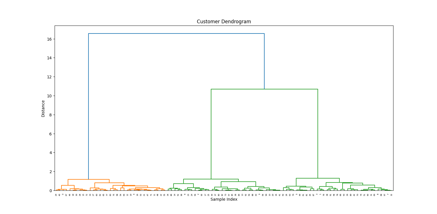

4. Interpreting results

From the dendrogram, we choose a height to "cut" and create three clusters:

labels = fcluster(linkage_matrix, t=3, criterion='maxclust')
plt.scatter(X_scaled[:, 0], X_scaled[:, 1], c=labels, cmap='rainbow')
plt.title('Customer Segments')
plt.xlabel('Feature 1')
plt.ylabel('Feature 2')
plt.show()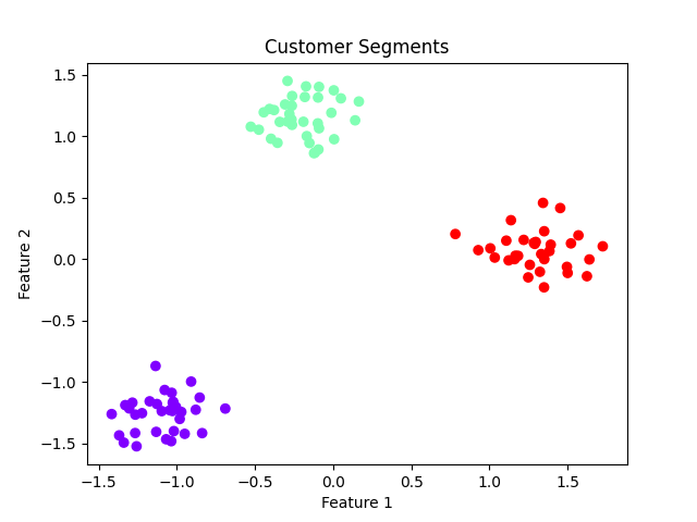

Business Implications:

• Clusters could represent customer groups such as budget-conscious, mid-tier, and premium customers.
• Enables personalized marketing and improved customer relationship strategies.

Hierarchical Clustering Advantages and Limitations

Choosing hierarchical clustering for your analysis has several advantages and limitations. 

Have a look below for some common ones:

Pros

• No need to specify the number of clusters: You can choose after visual inspection of the dendrogram.
• Intuitive visualization: Dendrograms help understand how clusters form.
• Flexible: Can handle various cluster shapes depending on linkage and distance metrics.

Cons

• Computationally intensive: Not ideal for large datasets.
• Sensitive to noise and outliers: A few outliers can significantly distort the dendrogram.
• No reassignment: Once a merge is done, it can’t be undone, which might lead to suboptimal clustering.

Conclusion

Hierarchical clustering is a versatile and interpretable clustering technique that is especially useful in exploratory data analysis and domains like genomics and customer segmentation. Despite its computational cost, its strength lies in the ability to uncover nested groupings and its flexibility in choosing the number of clusters post-hoc through dendrogram visualization.

For small to mid-sized datasets where interpretability is key, hierarchical clustering remains a go-to method for data scientists and analysts alike.

Want to learn more about the details of machine learning? Our Machine Learning Fundamentals in Python track and Introduction to Hierarchical Clustering in Python tutorial are all great places to start.