Variance Inflation Factor (VIF): Addressing Multicollinearity in Regression Analysis

What is Variance Inflation Factor (VIF)?

Developed by statistician Cuthbert Daniel, VIF is a widely used diagnostic tool in regression analysis to detect multicollinearity, which is known to affect the stability and interpretability of regression coefficients. More technically, VIF works by quantifying how much the variance of a regression coefficient is inflated due to correlations among predictors.

All of this is important because these correlations make it difficult to isolate the unique effect of each predictor on the target variable, leading to less reliable model estimates. I should also say that, in order to really tell the right story, VIF is always calculated for each predictor in a model.

The variance inflation factor formula

The VIF for a predictor X is calculated as:

Where:

• R² is the coefficient of determination obtained when X​ is regressed on all other predictors.

Step-by-step calculation

Finding VIF is a three-step process. The first step is to fit a separate linear regression model for each predictor against all other predictors. The second step is to obtain the R² value for each model. The final step is to calculate VIF using the formula above.

Interpretation of VIF Values

Here’s how to interpret VIF values to understand the level of multicollinearity:

• VIF = 1: This indicates no multicollinearity. The predictor is not correlated with other predictors, so it doesn’t inflate the standard error or affect the model’s stability.
• VIF between 1 and 5: This suggests moderate multicollinearity. There’s some correlation with other predictors, but it’s usually not severe. However, it’s worth keeping an eye on these predictors to see if multicollinearity becomes a problem, especially if other VIF values are high.
• VIF > 5: High multicollinearity is present. The predictor’s standard error may be noticeably inflated, which can make its coefficient less reliable. Consider taking steps to reduce multicollinearity, like removing or combining correlated predictors.
• VIF > 10: This signals serious multicollinearity. The predictor’s standard error is highly inflated, and its coefficient estimate is likely unstable. Corrective actions, such as removing the predictor or using regularization techniques, are usually needed.

For instance, if a predictor’s VIF is 10, it indicates that the variance of that predictor’s coefficient is 10 times what it would be if there were no multicollinearity. 

How the VIF Explains Multicollinearity in Regression

Multicollinearity causes standard errors to increase, which makes it harder to assess the significance of individual predictors. This happens because collinear variables carry similar information, making it difficult to separate their specific individual effects on the outcome variable. 

Although multicollinearity doesn’t necessarily harm the model’s ability to predict, it does reduce the reliability and clarity of the coefficients. This is especially problematic when we want to understand the individual impact of each predictor.

The variance inflation factor (VIF) serves as a precise diagnostic metric to identify multicollinearity. Unlike general observations about correlation, VIF isolates the combined effect of all predictors on each variable, highlighting interactions that might not be evident from pairwise correlations.

Variance Inflation Factor in Python and R

To make this actionable, let’s go through an example in both Python and R using a unique dataset. We’ll calculate VIF using automated packages and also using the VIF formula to build intuition. In order to have good practice, I have deliberately created a dataset where we will discover a high VIF value for one of our variables even though there isn't very high pairwise correlation between any two variables - so I think it's a compelling example. Let’s start with an overview of the dataset we’ll be using.

Dataset Overview:

This fictitious dataset represents survey results from a study conducted across 1,000 stores of a retail giant. Customers at each store were asked to rate various aspects of their shopping experience on a scale from -5 to +5, where -5 indicates a very negative experience, and +5 indicates a very positive experience. The average of the customer ratings at each store was taken across four key parameters:

• Ambience: Customer perception of the store's environment, such as cleanliness, layout, lighting, and overall atmosphere. 

• Customer_service: Rating of the service provided by store staff, including helpfulness, friendliness, and responsiveness to customer needs.

• Offers: Rating of the store's promotional offers, discounts, and deals available to customers.

• Product_range: Evaluation of the variety and quality of products available in the store.

The target variable, Performance, measures the overall performance of each store. However, it’s not relevant from the VIF perspective. You can download the dataset here. 

Variance inflation factor in Python

We’ll begin by calculating VIF values using the python packages. The first step is to load the dataset and the required libraries. 

from sklearn.linear_model import LinearRegression
from sklearn.metrics import r2_score
import pandas as pd
import numpy as np
import matplotlib.pyplot as plt
import seaborn as sns
from statsmodels.stats.outliers_influence import variance_inflation_factor
from statsmodels.tools.tools import add_constant

datacamp_retail_data = pd.read_csv(' vif_data.csv')
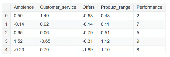
datacamp_retail_data.head()

The code above will load the data and display the first five records. 

As a next step, we can run a correlation matrix to check for pairwise correlation.

The code below selects four columns and stores them in a new DataFrame called correl_data. It then computes the pairwise correlation matrix using the .corr() function. The result is stored in the object, corr_matrix, which is a table showing the correlation coefficients between each pair of the selected columns. 

The matrix is then visualized using Seaborn's heatmap() function, displaying each correlation coefficient as a color-coded cell, where blue represents negative correlations and red represents positive correlations, based on the coolwarm color map. 

correl_data = datacamp_retail_data[['Ambience', 'Customer_service', 'Offers', 'Product_range']]

# Compute the pairwise correlation matrix
corr_matrix = correl_data.corr()

# Visualize the correlation matrix
plt.figure(figsize=(10, 8))
sns.heatmap(corr_matrix, annot=True, cmap='coolwarm', vmin=-1, vmax=1)
plt.title('Pairwise Correlation Matrix')
plt.show()

Output:

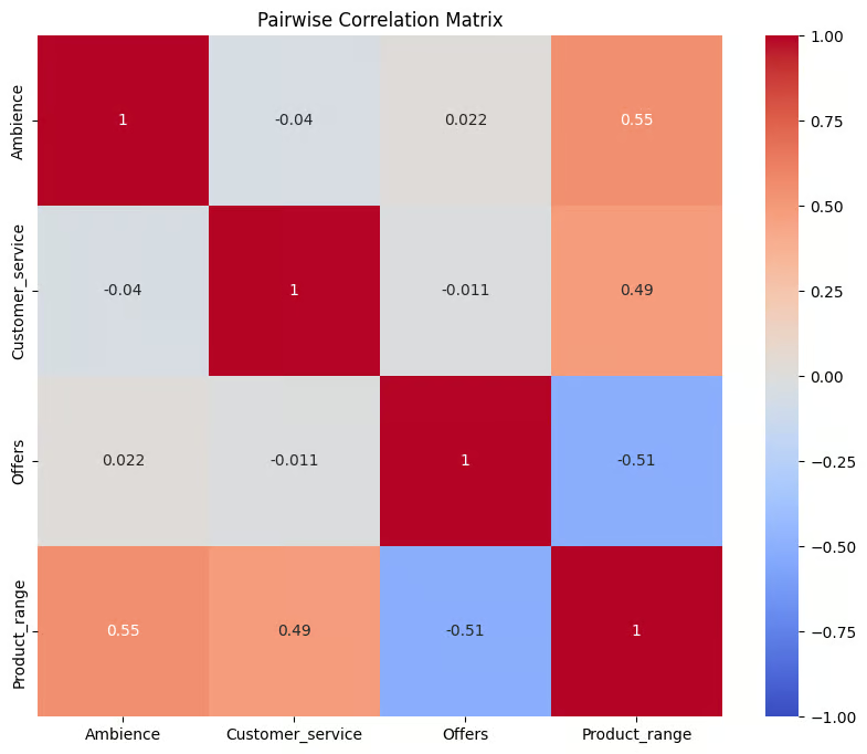
  Correlation between the variables. Image by Author

The plot provides a visual summary of relationships between variables in correl_data. The correlation values range from -1 to 1, where values closer to 1 indicate a strong positive correlation, values closer to -1 indicate a strong negative correlation, and values around 0 suggest no correlation. It is evident that there is no strong pairwise correlation amongst the variables, with none of the correlation values being greater than even 0.6. 

The next step is to calculate the VIF values for the predictor variables. The code below calculates the values for each predictor variable in the dataset to check for multicollinearity. 

First, it defines X by removing the target column Performance and adding an intercept. Then, it creates a DataFrame, datacamp_vif_data,  to store the predictor names and their VIF values. Using a loop, it then calculates the VIF for each predictor with the variance_inflation_factor() function, where higher VIFs indicate presence of multicollinearity. 

# Define the predictor variables
X = datacamp_retail_data.drop(columns=['Performance'])

# Add a constant to the model (intercept)
X = add_constant(X)

# Calculate VIF for each feature
datacamp_vif_data = pd.DataFrame()
datacamp_vif_data['Feature'] = X.columns
datacamp_vif_data['VIF'] = [variance_inflation_factor(X.values, i) for i in range(X.shape[1])]
print(datacamp_vif_data)

Output:

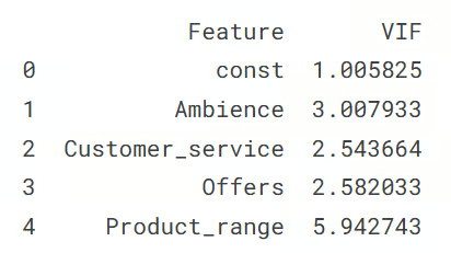
Output showing the VIF values. Image by Author

This output shows the VIF value for each predictor variable, indicating multicollinearity levels in the dataset. The const row represents the intercept term, with a VIF close to 1, meaning it has no multicollinearity. Among the predictor variables, Product_range has the highest VIF (5.94), which suggests that it needs corrective measures. All the other predictors have VIF values below 3, indicating low multicollinearity. 

Manual approach to VIF calculation

The other approach is to calculate the values seperately by regressing each independent variable against the other predictor variables.  

So how it works is that for each feature in retail_data, it sets that feature as the dependent variable (y) and the remaining features as independent variables (X). A linear regression model is then fitted to predict y using X, and the R-squared value of the model is used to calculate VIF using its formula we discussed in the initial section.

Subsequently, each feature and its corresponding VIF values are stored in a dictionary (vif_manual), which is then converted to a DataFrame (vif_manual_df) for display. 

datacamp_retail_data = retail_data.drop(columns=['Performance'])

# Manual VIF Calculation
vif_manual = {}

for feature in retail_data.columns:
    # Define the target variable (current feature) and predictors (all other features)
    y = datacamp_retail_data[feature]
    X = datacamp_retail_data.drop(columns=[feature])

    # Fit the linear regression model
    model = LinearRegression().fit(X, y)

    # Calculate R-squared
    r_squared = model.score(X, y)

    # Calculate VIF
    vif = 1 / (1 - r_squared)
    vif_manual[feature] = vif

# Convert the dictionary to a DataFrame for better display
vif_manual_df = pd.DataFrame(list(vif_manual.items()), columns=['Feature', 'VIF'])
print(vif_manual_df)

 Output:

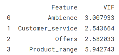
Output showing the VIF values. Image by Author

The output shows each feature along with its VIF value, helping to identify potential multicollinearity issues. You can see the result is obviously the same as we got above; and so will be its interpretation, which is that the Product_range variable is exhibiting multicollinearity.

Variance inflation factor in R

In this section, we’ll repeat the exercise of the above variance inflation factor in the Python section, especially for developers who work with the R programming language. We start by loading the dataset and the necessary libraries.

library(tidyverse)
library(car)
library(corrplot)

data <- read.csv('vif_data.csv')
str(data)

Output:

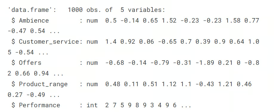
The next step is to compute the pairwise correlation matrix, and visualize it with the heatmap. The cor() and corrplot functions help us accomplish this task.

# Remove the target column
predictors_data <- data[, !(names(data) %in% "Performance")]

# Calculate the correlation matrix
correlation_matrix <- cor(predictors_data)

# Plot the correlation heatmap
# Load necessary libraries
library(ggplot2)
library(reshape2)
melted_corr_matrix <- melt(correlation_matrix)

# Plot the heatmap with ggplot2
ggplot(data = melted_corr_matrix, aes(x = Var1, y = Var2, fill = value)) +
  geom_tile(color = "white") +
  scale_fill_gradient2(low = "blue", high = "red", mid = "white", 
                       midpoint = 0, limit = c(-1, 1), space = "Lab", 
                       name="Correlation") +
  theme_minimal() + # Minimal theme for a clean look
  theme(axis.text.x = element_text(angle = 45, vjust = 1, hjust = 1)) +
  labs(x = "", y = "") + # Remove axis labels
  geom_text(aes(Var1, Var2, label = round(value, 2)), color = "black", size = 4) +
  theme(axis.text=element_text(size=15))

Output:

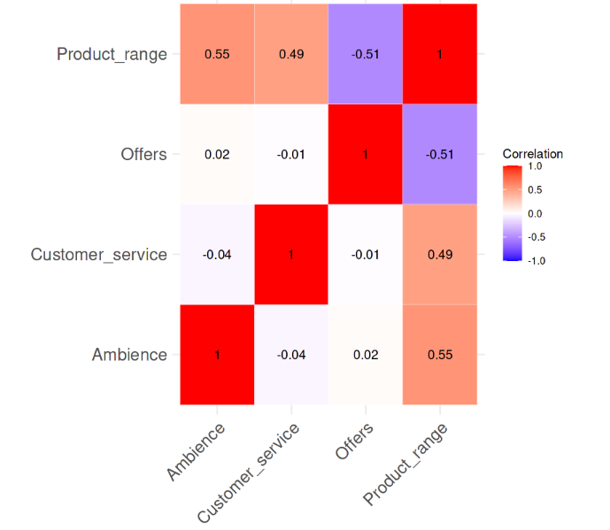
Correlation between the variables. Image by Author

It is evident from the correlation heatmap that there is no strong pairwise-correlation amongst the variables, with none of the correlation values even being greater than 0.6. Now, we’ll compute the VIF values and see if there is anything alarming. The following line of code does that task. 

# Fit a regression model
model <- lm(Performance ~ Ambience + Customer_service + Offers + Product_range, data = data)

# Calculate VIF
vif(model)

Output:

From the output, we can see that amongst the predictor variables, only the Product_range variable has the VIF value greater than 5, which suggests high multicollinearity that needs corrective measures. 

Manual Approach to VIF Calculation

The other approach to VIF calculation would be to calculate the VIF values for each variable seperately by regressing each independent variable against the other predictor variables.  

This is performed in the code below, which uses the sapply()function across each predictor, where each predictor is set as the dependent variable in a linear regression model with the other predictors as independent variables. 

The R-squared value from each model is then used to calculate the VIF values with its formula. Finally, the result, vif_values, displays the VIF for each predictor, helping identify multicollinearity issues.

# VIF calculation for each predictor manually
predictors <- c("Ambience", "Customer_service", "Offers", "Product_range")

vif_values <- sapply(predictors, function(pred) {
    formula <- as.formula(paste(pred, "~ ."))
    model <- lm(formula, data = data[, predictors])
    1 / (1 - summary(model)$r.squared)
})

print(vif_values)

Output:

We get the same result and it’s evident that the variable Product_range with a high VIF value above 5 needs intervention. 

VIF vs. Correlation Matrix and Other Methods

As a recap, here are the popular methods to detect multicollinearity:

• High VIF Values: A high VIF value is a clear indicator of multicollinearity. When these values exceed certain thresholds, they indicate that a predictor is strongly related to other predictors, which can affect the stability, reliability and performance of the model.
• Correlation Matrices: By examining a correlation matrix, you can see the pairwise correlations between predictors. High pairwise correlations suggest multicollinearity between those specific predictors. However, this method only detects direct linear relationships between two variables and may miss multicollinearity involving more complex interactions among several variables.
• Coefficient Changes: If the coefficients of predictors change significantly when you add or remove other variables from the model, this can be a sign of multicollinearity. Such fluctuations indicate that certain predictors may be sharing common information, making it harder to identify each variable’s unique impact on the outcome.

Amongst all of these methods, VIF is particularly useful because it can detect multicollinearity even when pairwise correlations are low, as we saw in our own example. This makes VIF a more comprehensive tool.

Additional Ideas on How to Address High VIF Values

If VIF values indicate high multicollinearity, and you don't necessarily just want to remove the variable, there are some other, more advanced strategies to mitigate multicollinearity:

1. Feature Selection: Remove one of the highly correlated predictors, and recalculate the VIF to see if it helps simplify the model and improve stability.
2. Principal Component Analysis (PCA): Use PCA to combine your predictors into a smaller set of uncorrelated components. This transforms the original variables into new, independent, and uncorrelated ones that capture most of the data's variation, helping to address multicollinearity without losing valuable information.
3. Regularization Techniques: Apply ridge or lasso regression, which add penalty terms to the model. These techniques help reduce multicollinearity by shrinking the influence of correlated variables, making the model more stable and reliable.

Conclusion

Knowing how to use VIF is key to identifying and fixing multicollinearity, which improves the accuracy and clarity of regression models. Regularly checking VIF values and applying corrective measures when needed helps data professionals and analysts build models they can trust. This approach ensures that each predictor’s effect is clear, making it easier to draw reliable conclusions from the model and make better decisions based on the results. Take our Machine Learning Scientist in Python career track to really understand how to build models and use them. Plus, the completion of the program looks great on a resume.

Also, for further learning, consider exploring the following resources from the DataCamp blog and tutorial sections:

• Essentials of Linear Regression in Python: Learn what formulates a regression problem and how a linear regression algorithm works in Python.
• How to Do Linear Regression in R: Learn linear regression, a statistical model that analyzes the relationship between variables using R.
• QR Decomposition in Machine Learning: A Detailed Guide: Learn about QR decomposition, the matrix factorization technique that decomposes matrix A into the product of an orthogonal matrix Q and an upper triangular matrix R.
• Lasso and Ridge Regression in Python Tutorial: Learn about the lasso and ridge techniques of regression. Compare and analyze the methods in detail.