Weibull Distribution: How to Model Time-to-Event Data

When you're analyzing how long things last (whether it's the lifespan of electronic components, patient survival times, or equipment reliability), you need a distribution that can handle the complexity of failure patterns. The Weibull distribution doesn't assume failures happen at a constant rate like simpler models do. Instead, it can model scenarios where failure rates increase over time (like wear-out processes), decrease initially (like early manufacturing defects being weeded out), or remain steady.

If probability concepts are new to you, our Foundations of Probability in R course covers the statistical basics you'll need for advanced distribution work. This tutorial will guide you through the mathematical foundations of the Weibull distribution. You'll learn how to estimate its parameters from data and see how its flexibility makes it particularly useful in reliability analysis and survival studies. By the end, you'll understand not just the theory behind this useful distribution, but also when and how to apply it to your own time-to-event analysis challenges.

What Is the Weibull Distribution?

The Weibull distribution is a continuous probability distribution designed for modeling time-to-event data. You'll encounter it most often in failure analysis, survival studies, and reliability engineering where understanding "when something happens" is the goal. 

What sets the Weibull apart from simpler alternatives is its adaptability to different failure patterns. While some distributions assume events occur at steady, predictable rates, the Weibull can handle situations where the likelihood of events changes over time. This flexibility makes it useful when you're working with complex systems or processes where the underlying mechanisms aren't fully understood.

Historical Context and Fundamental Principles

The story behind this distribution begins with Swedish mathematician Waloddi Weibull, who developed it in the 1930s while studying material strength and fatigue. His work laid the foundation for modern reliability engineering.

The distribution comes in two primary forms that serve different analytical needs. The two-parameter Weibull uses shape and scale parameters to model scenarios where events can begin immediately. The three-parameter version adds a location parameter, creating a minimum threshold before events can occur—useful for modeling systems with built-in delays or "burn-in" periods.

The Weibull belongs to a family of related distributions, with the exponential distribution appearing as a special case. This connection helps explain why you'll often see Weibull and exponential models compared in reliability contexts. Weibull's broader flexibility allows it to approximate other well-known distributions under specific parameter conditions, which contributes to its widespread adoption.

Parameters of the Weibull Distribution

Now that we've covered the historical development and basic behavior, let's explore the parameters that give the Weibull distribution its flexibility. Each parameter tells you something specific about how your data behaves.

The shape parameter (k or β) controls the distribution's character and how the hazard function behaves. When values are less than 1, you're looking at infant mortality patterns where early failures happen due to manufacturing defects. When values are greater than 1, you see wear-out failures where things break down from regular use over time.

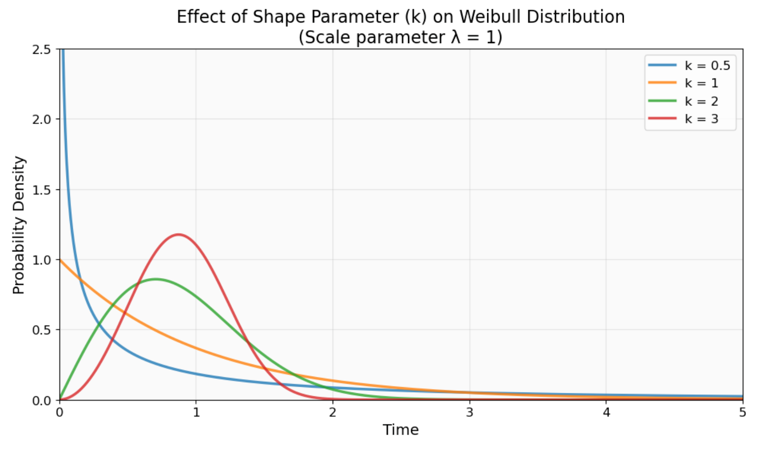
Effect of shape parameter (k) on Weibull distribution behavior. Notice how k < 1 creates high early failure probability (blue curve), k = 1 produces constant failure rates (orange), and k > 1 shows increasing failure rates over time (green and red curves). Image by Author.

The scale parameter (λ or η) represents the characteristic life. This is the time when exactly 63.2% of items will have failed, regardless of the shape parameter value. You can view this as the distribution's typical lifespan, though the actual mean might differ because of the distribution's shape.

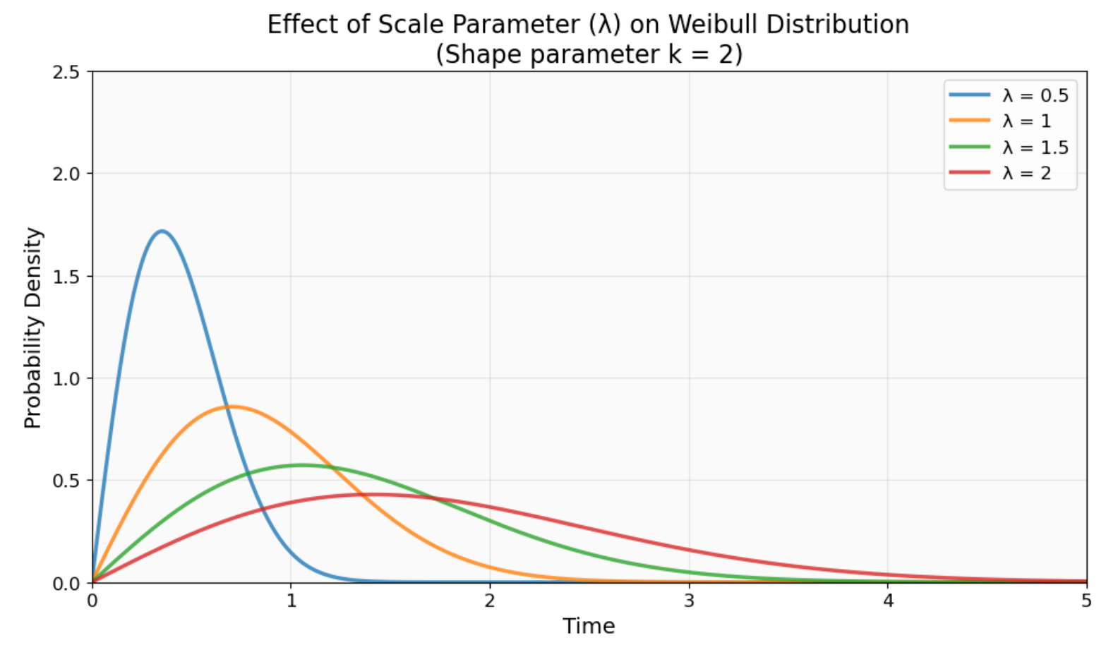
How the scale parameter (λ) shifts the Weibull distribution along the time axis. Larger λ values stretch the distribution rightward (longer characteristic life), while smaller values compress it leftward (shorter characteristic life). The shape remains consistent. Image by Author.

In three-parameter applications, the location parameter (θ or γ) shifts the distribution along the time axis. It represents a guaranteed minimum lifetime before any failures can begin, which helps when you're modeling systems with burn-in periods or components with warranty periods where early failure is impossible.

Different fields use different notations, so you might see (k,λ) in reliability engineering or (β,η) in survival analysis. The mathematical relationships stay the same regardless of which notation you encounter.

Mathematical Characterization and Statistical Properties

The Weibull distribution's mathematical foundation provides the tools needed for practical applications. Let's explore the core functions that make this distribution useful.

Core functions and metrics

The probability density function (PDF) describes the likelihood of failure occurring at any specific time. For the Weibull distribution, this is:

This function shows how failure probability density changes over time, with the shape parameter k determining if failures are more likely early (k < 1), constant over time (k = 1), or increasing with age (k > 1).

The cumulative distribution function (CDF) gives the probability that failure occurs by a specific time:

This function works well for calculating the percentage of items expected to fail within a given timeframe. The reliability function (1-CDF) provides the complementary perspective, showing the probability of survival beyond time t.

The hazard function reveals the instantaneous failure rate at any given time:

This function is essential for understanding how risk changes over time. When k < 1, the hazard decreases (improving reliability), when k = 1, it remains constant, and when k > 1, it increases (deteriorating reliability). The survival function, identical to the reliability function, represents the probability of surviving beyond a given time.

Statistical moments characterize the distribution's central tendencies and variability. The mean involves the gamma function and depends on both parameters, making it more complex than the characteristic life. The variance quantifies spread around the mean, while the median often provides more intuitive interpretation than the mean for skewed distributions. The mode represents the most likely failure time, though it may not exist for all parameter combinations.

The moment generating function captures all statistical moments in a single expression, while entropy measures the uncertainty or information content of the distribution. These properties, along with failure rate behavior patterns, make the Weibull distribution suitable for modeling diverse real-world phenomena where simple exponential assumptions prove inadequate.

Conditional reliability and percentiles

Conditional reliability calculations answer practical questions like "If this component has already survived 1000 hours, what's the probability it will last another 500 hours?" This involves calculating the probability of survival for an additional period given survival to the current point. The calculation uses the following relationship:

where R(t) is the reliability function.

Percentiles help estimate important lifetime metrics that drive business decisions. The B₁₀ life represents the time when 10% of items will have failed, while B₉₀ life indicates when 90% of items will have failed. These percentiles are essential for warranty analysis, maintenance planning, and risk assessment.

The percent point function (inverse CDF) provides direct quantile estimation by solving F(t) = p for any desired probability p. This function transforms cumulative probabilities back into time values, enabling you to determine specific failure times for given reliability levels. Most statistical software packages include built-in functions for these calculations, making percentile estimation straightforward once you've estimated the Weibull parameters.

Parameter Estimation Methodologies

Understanding the mathematical properties is one thing, but how do you actually determine these parameters from your data? Estimating Weibull parameters from data requires choosing the right method for your situation and data characteristics. Each approach has distinct advantages and limitations.

Maximum likelihood estimation (MLE)

MLE provides the most statistically rigorous approach for parameter estimation. It finds parameter values that maximize the likelihood of observing your actual data, making it effective with complete datasets. Think of it as finding the parameters that make your observed data "most likely" to have occurred.

The method handles censored data (where you know items survived to a certain point but not their exact failure times) through specialized algorithms. This is useful in reliability testing where you can't always wait for every item to fail. ​​Most statistical software packages include MLE routines specifically designed for Weibull analysis. While computational complexity increases with dataset size, modern implementations handle datasets with hundreds of thousands of observations efficiently.

Method of moments (MOM)

The MOM approach estimates parameters by matching theoretical moments to sample moments from your data. While less statistically efficient than MLE, it offers computational simplicity and often provides good starting estimates for more complex methods.

This approach works well when you need quick estimates or when dealing with data that doesn't fit MLE assumptions perfectly. It's also helpful for getting a rough sense of your parameters before diving into more sophisticated analysis.

Least squares and graphical techniques

Weibull probability plots transform data onto logarithmic coordinates where Weibull distributions appear as straight lines, allowing you to visually validate model fit while estimating parameters through linear regression. The method uses specially scaled graph paper (now digitally reproduced in software) with a double-logarithmic transformation that linearizes the Weibull cumulative distribution function.

The process involves ranking your failure data from smallest to largest, calculating median rank positions for each data point (which estimate the cumulative failure probability), and plotting failure times against these probabilities. If your data follows a Weibull distribution, the points will form approximately a straight line whose slope equals the shape parameter and whose position determines the scale parameter. It's old-school, but it works and the visual feedback is valuable for understanding your data. When points deviate significantly from linearity, it suggests the Weibull model may not be appropriate for your dataset, making this technique valuable for both parameter estimation and model validation.

Three-parameter challenges

Estimating the location parameter θ presents unique difficulties because it affects the distribution's lower bound. Standard MLE can produce unreliable estimates when θ approaches the minimum observed failure time.

Profile likelihood methods address these estimation issues by treating θ as a nuisance parameter, providing more stable estimates for the shape and scale parameters. It's a bit more complex, but often necessary for reliable results.

Applications Across Disciplines

The Weibull distribution's versatility shines through its applications across diverse fields. Each domain leverages specific aspects of the distribution's flexibility.

Reliability engineering

Reliability engineers use Weibull analysis for accelerated life testing, where products are tested under stress conditions to predict normal-use lifetimes. Instead of waiting years to see how long something lasts, you can stress-test it and extrapolate to normal conditions.

Warranty analysis relies on Weibull models to estimate future claims and set appropriate coverage periods. Companies need to know how many products will fail within warranty periods to price their products correctly.

Preventive maintenance scheduling benefits from Weibull's ability to model changing failure rates over equipment lifecycles. Unlike exponential models that assume constant failure rates, Weibull can tell you when failure rates start increasing, helping you time maintenance before things break down.

Medical and biological sciences

Survival analysis in medical research frequently employs Weibull models to study treatment efficacy and patient prognosis. The distribution naturally handles censored data common in clinical trials where patients may leave the study before experiencing the event of interest.

Weibull regression extends basic analysis by incorporating patient characteristics (age, treatment type, disease stage) as covariates. This provides personalized survival estimates essential for treatment planning, helping doctors give patients realistic expectations about their prognosis.

Material science and forestry

Materials engineers use Weibull distributions to model the strength of brittle materials like ceramics and composites, where the weakest link determines overall failure. The distribution's ability to model extreme values makes it ideal for these applications where you care about the worst-case scenario.

Forest management applies Weibull models to tree diameter distributions, helping predict harvest yields and plan sustainable forestry operations. It's a practical application that helps balance economic and environmental concerns.

Wind energy and environmental studies

While this article focuses on time-to-event applications, Weibull distributions also model other phenomena in environmental engineering. Wind resource assessment uses Weibull to characterize wind speed patterns at potential turbine sites, where shape parameters indicate wind consistency for energy production planning.

Advanced Topics and Extensions

As useful as these standard applications are, modern problems often require pushing beyond basic Weibull analysis. 

Model selection and goodness-of-fit

Choosing between Weibull and alternative distributions requires systematic testing using goodness-of-fit statistics like the Kolmogorov-Smirnov and Anderson-Darling tests. These tests quantify how well your chosen distribution matches observed data patterns, giving you confidence in your model choice.

Graphical diagnostics complement statistical tests by revealing patterns that numbers alone might miss. Residual analysis helps identify systematic deviations from expected behavior, while information criteria (AIC/BIC) balance model fit against complexity. You basically want a model that fits well without being unnecessarily complicated.

Regression and mixture models

Weibull regression incorporates explanatory variables directly into the distribution parameters, allowing you to model how factors like temperature, load, or patient characteristics affect failure behavior. This extension is useful in reliability testing and medical research where multiple factors influence outcomes.

Mixture Weibull models handle populations with distinct subgroups (like different failure modes) by combining multiple Weibull distributions. Think of a population where some items fail from wear-out while others fail from random defects. You need different models for each failure mode.

Machine learning applications increasingly use these models for complex pattern recognition and neural network applications, bridging traditional statistical methods with modern AI techniques.

Competing risks and degradation models

Some systems will face multiple failure modes simultaneously. Mechanical wear, electrical failure, and environmental degradation might all threaten the same component. Competing risks models use multiple Weibull distributions to represent each failure mode, helping you understand which risks are most critical.

Degradation models track how system performance declines over time, using Weibull distributions to model the time until performance drops below acceptable thresholds. This is useful for systems where you can measure degradation before complete failure occurs.

Related and special forms

The inverse Weibull distribution models situations where larger values are less likely to occur, such as minimum strength in materials or shortest survival times in biology. This variant is useful when traditional Weibull assumptions don't fit your data patterns.

Discrete Weibull distributions adapt the continuous model for count data, such as the number of cycles until failure or discrete time intervals in survival studies. It's not as common, but handy when your data comes in discrete chunks rather than continuous measurements.

Conclusion

The Weibull distribution's adaptability makes it valuable for analyzing when things happen over time. It handles increasing, decreasing, or steady hazard rates and works well with incomplete data. Our Survival Analysis in Python and Survival Analysis in R courses let you practice with datasets and established methods.

Future research directions include Bayesian approaches that incorporate prior knowledge more effectively, machine learning hybrids that combine Weibull modeling with neural networks, and big data applications that scale traditional methods to massive datasets.