Cauchy Distribution: Understanding Heavy-Tailed Data

The Cauchy distribution poses an intriguing statistical puzzle. While it shares the familiar bell-curved shape with many other continuous probability distributions, it defies conventional analysis by lacking both a defined mean and variance. Named after mathematician Augustin-Louis Cauchy, this distribution emerges naturally in fields ranging from financial modeling to Bayesian statistics.

As a teaching tool, the Cauchy distribution illustrates fundamental statistical concepts with remarkable clarity. It demonstrates the non-convergence of sample means, highlights the importance of distributional assumptions, and shows how estimators perform under varying conditions.

Looking to master these statistical concepts and their applications in data science? Explore our Machine Learning Scientist in R career track, where you'll learn to implement these ideas using R programming.

What Is the Cauchy Distribution?

The Cauchy distribution is a continuous probability distribution that's famous for its unique properties and heavy tails. It's characterized by two key parameters:

1. Location Parameter (θ): This parameter determines where the peak (or center) of the distribution lies on the x-axis. Think of it as shifting the entire distribution left or right without changing its shape.
2. Scale Parameter (σ): This parameter controls how spread out the distribution is. Larger values of σ create wider, flatter distributions with heavier tails. You can think of it as stretching or squeezing the distribution horizontally.

The distribution is mathematically defined by its probability density function (PDF):

When we set θ = 0 and σ = 1, we get what's called the standard Cauchy distribution. This is the simplest form of the distribution and serves as a reference point for understanding more complex cases.

The Main Characteristics of the Cauchy Distribution

The defining properties of Cauchy distributions

Heavy tails

Think of the Cauchy distribution as the "extreme events" distribution. While a normal distribution suggests that values far from the center are very rare (like finding a person who is 7 feet tall), the Cauchy distribution tells us that extreme values occur more frequently than you might expect. 

For example, in stock market returns, massive single-day price changes (like during market crashes or rallies) happen more often than a normal distribution would predict. The Cauchy distribution's heavy tails can better capture these "black swan" events.

Undefined mean and variance

This is perhaps the most fascinating property of the Cauchy distribution. Unlike most distributions you've encountered, the Cauchy distribution doesn't have a meaningful average (mean) or spread (variance). 

To understand why this matters: if you take repeated samples from a Cauchy distribution and try to calculate their average, you won't converge to any specific value, even with millions of samples. This has implications for statistical analysis, as traditional statistical methods that rely on means and variances (like t-tests or ANOVA) don't work with Cauchy-distributed data.

Symmetry

The Cauchy distribution is perfectly balanced around its location parameter (θ), like a mirror image on both sides. However, this symmetry doesn't mean it behaves like the familiar normal distribution. While both distributions are symmetric, the Cauchy distribution spreads its probability much more widely. This means that even though it has a clear center, values can stray very far from this center with significant probability.

Stability

The Cauchy distribution has a remarkable property: when you add together two independent Cauchy-distributed variables, you get another Cauchy distribution! This property, known as stability, is shared with only a few other distributions (like the normal distribution). It is particularly useful in physics and financial modeling, where we often need to understand how combined random processes behave over time.

Things to notice when using the Cauchy distribution

Handling outliers

The Cauchy distribution excels at handling outliers because it expects them to occur. This makes it particularly useful in scenarios where extreme values are natural parts of the data, not mistakes to be removed. In these cases, traditional outlier detection methods might be too aggressive, inappropriately flagging legitimate data points for removal. The Cauchy distribution provides a framework for building robust models that won't be unduly influenced by extreme observations, making it a valuable tool when working with datasets where outliers are an inherent feature rather than an anomaly to be eliminated.

Model selection

Choosing whether to use a Cauchy distribution depends on your data and goals. The Cauchy distribution is particularly valuable when your data frequently shows extreme values, when you're working with ratios of normally distributed variables, or when you need a robust model that can handle heavy-tailed data. However, you should be cautious about using the Cauchy distribution in certain situations: when you need to rely on means and variances, when your data actually follows a lighter-tailed distribution, or when computational efficiency is a primary concern. Understanding these trade-offs is helpful for making informed decisions about whether the Cauchy distribution is appropriate for your specific analysis needs.

Computational efficiency

While the Cauchy distribution's mathematical formula is straightforward, working with it computationally can be challenging. Parameter estimation often requires specialized techniques like Markov Chain Monte Carlo (MCMC), and standard maximum likelihood methods may struggle with the heavy tails. Fortunately, modern statistical software packages often include specific tools for handling Cauchy distributions, making it more feasible to work with this distribution in practice despite its computational complexities.

Mathematical Properties of the Cauchy Distribution

The Cauchy distribution possesses several important mathematical properties that make it unique and useful:

• A stable distribution with an interesting behavior: when you add two Cauchy-distributed variables together, you get another Cauchy distribution with scaled parameters. This makes it useful in studying cumulative effects in physics and finance.
• Undefined moments, including mean and variance, which makes it a fascinating counterexample in probability theory. This property helps students understand why the Central Limit Theorem requires finite variance.
• An elegantly simple mathematical form, with a straightforward PDF and characteristic function. Despite its complex behavior, its basic mathematical description is surprisingly tractable.
• The ratio property: if you divide one normal random variable by another independent normal random variable, you get a Cauchy distribution. This makes it naturally suited for modeling ratios and proportions.
• Strong Bayesian applications, particularly as a prior distribution in hierarchical models. Its heavy tails make it an excellent choice for scale parameters where robustness is important.

Visualizing the Cauchy Distribution in R and Python

The Cauchy distribution's behavior is best understood through visualization. Let's use R to create plots of different Cauchy distributions, demonstrating how the location (θ) and scale (σ) parameters affect the shape and position of the distribution.

Cauchy distribution in R

R provides functions for working with Cauchy distributions through its stats package. We'll also use ggplot2 for creating clear, publication-quality visuals:

# Load required libraries
library(ggplot2)  # for plotting
# Note: dcauchy is from the stats package which is loaded by default in R

# Create a sequence of x values
x <- seq(-10, 10, length.out = 1000)

# Generate different Cauchy distributions using stats::dcauchy
# Standard Cauchy (θ = 0, σ = 1)
standard_cauchy <- dcauchy(x, location = 0, scale = 1)

# Location and Scale Adjusted (θ = 2, σ = 3)
adjusted_cauchy <- dcauchy(x, location = 2, scale = 3)

# Highly Scaled (θ = -1, σ = 5)
scaled_cauchy <- dcauchy(x, location = -1, scale = 5)

# Create a data frame for plotting
plot_data <- data.frame(
  x = rep(x, 3),
  density = c(standard_cauchy, adjusted_cauchy, scaled_cauchy),
  distribution = rep(c("Standard (θ=0, σ=1)", 
                      "Adjusted (θ=2, σ=3)", 
                      "Scaled (θ=-1, σ=5)"), 
                    each = length(x))
)

# Create the plot
ggplot(plot_data, aes(x = x, y = density, color = distribution)) +
  geom_line(size = 1) +
  theme_minimal() +
  labs(title = "Comparison of Cauchy Distributions",
       x = "x",
       y = "Density",
       color = "Parameters") +
  theme(legend.position = "bottom",
        plot.title = element_text(hjust = 0.5)) +
  scale_color_brewer(palette = "Set1")

This code generates a comparison plot of three different Cauchy distributions:

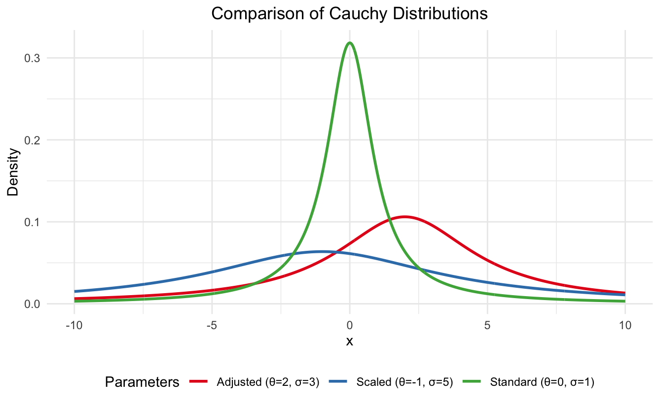
Cauchy distribution in R. Image by Author

1. Standard Cauchy (green line): With θ = 0 and σ = 1, this represents the baseline case. Notice its sharp peak at x = 0 and symmetric heavy tails.
2. Location-Adjusted Cauchy (red line): Setting θ = 2 shifts the peak to the right while maintaining the shape. This demonstrates how the location parameter affects the center of the distribution without changing its spread.
3. Highly-Scaled Cauchy (blue line): With θ = -1 and σ = 5, this shows a shifted and much flatter distribution. The larger scale parameter creates wider, heavier tails and reduces the peak height, illustrating how σ controls the spread.

The visualization clearly shows how increasing the scale parameter (σ) leads to a flatter, more spread-out distribution, while the location parameter (θ) simply shifts the entire distribution left or right.

Cauchy distribution in Python

After exploring the Cauchy distribution's parameters in R, let's use Python to compare the Cauchy distribution with its more familiar cousin, the Normal distribution. Python's scientific computing stack, particularly scipy.stats, provides excellent tools for working with probability distributions.

While R's stats package gave us direct access to Cauchy distribution functions, Python's scipy.stats module offers similar functionality with a slightly different interface. We'll use matplotlib, Python's primary plotting library, to create a clear visualization:

import numpy as np
import matplotlib.pyplot as plt
from scipy import stats

# Set style parameters for better visualization
plt.style.use('seaborn')
plt.rcParams.update({
    'font.size': 16,
    'axes.labelsize': 18,
    'axes.titlesize': 24,
    'xtick.labelsize': 16,
    'ytick.labelsize': 16,
    'legend.fontsize': 16,
})

# Create data
x = np.linspace(-10, 10, 1000)
cauchy = stats.cauchy.pdf(x, loc=0, scale=1)
normal = stats.norm.pdf(x, loc=0, scale=1)

# Create the plot
plt.figure(figsize=(12, 8))

# Plot distributions
plt.plot(x, cauchy, 'b-', linewidth=2.5, label='Cauchy(0,1)')
plt.plot(x, normal, 'r--', linewidth=2.5, label='Normal(0,1)')

# Customize the plot
plt.title('Cauchy vs Normal Distribution', pad=20)
plt.xlabel('x', labelpad=10)
plt.ylabel('Density', labelpad=10)

# Customize legend
plt.legend(fontsize=16, bbox_to_anchor=(0.99, 0.99), 
          loc='upper right', borderaxespad=0.)

# Add grid and adjust layout
plt.grid(True, alpha=0.3)
plt.tight_layout()

plt.show()

The code above creates a comparison between the standard Cauchy distribution (blue solid line) and the standard Normal distribution (red dashed line), both centered at 0 with a scale parameter of 1.

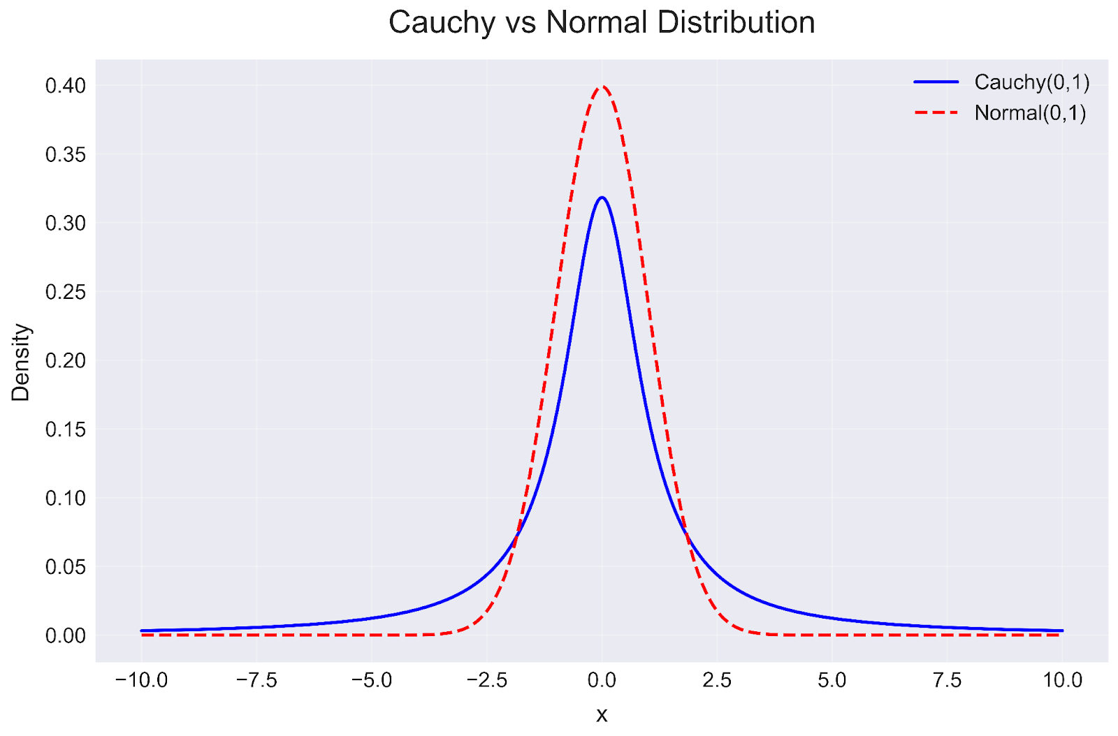
Cauchy distribution in Python. Image by Author

This visualization reveals several key insights:

1. Peak Height: The Normal distribution reaches a higher peak density (approximately 0.4) compared to the Cauchy distribution (approximately 0.32), indicating that values are more concentrated around the center in the Normal distribution.
2. Heavy Tails: Notice how the Cauchy distribution's blue line remains higher than the Normal distribution's red dashed line as we move away from the center. These "heavy tails" mean that extreme values are much more likely under a Cauchy distribution than a Normal distribution.
3. Practical Implications: The heavier tails of the Cauchy distribution make it more suitable for modeling phenomena where extreme events occur more frequently than would be predicted by a Normal distribution, such as financial market returns or certain physical phenomena.

This comparison helps explain why the Cauchy distribution is often used in scenarios where the Normal distribution underestimates the probability of extreme events. While both distributions are symmetric around their center, the Cauchy distribution's heavy tails make it more appropriate for modeling systems where outliers are common rather than rare exceptions.

When the Cauchy Distribution is Useful

The Cauchy distribution serves specific purposes in data analysis and modeling. Let's examine how it's used effectively across different domains.

Finance: Managing market uncertainty

Modeling returns

Financial markets are known for their unpredictable nature, often experiencing dramatic price swings that would be considered "impossible" under normal distribution assumptions. The Cauchy distribution shines here because:

• It naturally captures "black swan" events like market crashes or sudden rallies.
• It better reflects the reality that extreme market movements happen more frequently than traditional models predict.
• It doesn't underestimate the risk of large price movements.

For example, during the 2008 financial crisis, many traditional models failed because they assumed normal distributions. A Cauchy-based model would have better anticipated the possibility of such extreme market movements.

Risk assessment

When evaluating investment risks, the Cauchy distribution provides a more conservative and realistic view. It helps risk managers set more appropriate capital reserves by accounting for extreme scenarios, better estimates the probability of significant losses or gains, and provides a more realistic model for stress testing portfolios. This approach to risk assessment helps financial institutions prepare for unlikely but impactful market events.

Bayesian statistics: Robust statistical inference

Prior distributions

In Bayesian analysis, choosing the right prior distribution is critical. The Cauchy distribution is particularly valuable here because:

• Its heavy tails make it less likely to accidentally rule out important parameter values
• It's especially useful for scale parameters (like standard deviations) in hierarchical models
• It helps prevent the model from being overly confident in its estimates

For example, when analyzing the effectiveness of a new medical treatment, using a Cauchy prior for the effect size helps ensure we don't underestimate the possibility of large treatment effects.

Robust regression

Traditional regression can be heavily influenced by outliers. Using Cauchy-distributed error terms helps build more robust models by making the model less sensitive to extreme observations. The results remain reliable even when data contains outliers, and predictions are more stable in the presence of unusual data points. This robustness makes Cauchy-distributed error terms particularly valuable when working with real datasets that often contain unexpected or extreme values.

Machine learning and data science: Building resilient models

Robust algorithms

Modern machine learning often deals with noisy, real-world data. The Cauchy distribution helps build more resilient algorithms by:

• Providing a better model for noise in sensor data
• Helping handle outliers in training data without removing them
• Making learning algorithms more robust to corrupted data points

For example, in computer vision, using Cauchy-distributed noise models can help algorithms better handle image artifacts or sensor glitches.

Generative models

In advanced machine learning applications, the Cauchy distribution helps create more flexible models. It's useful in variational autoencoders where data might have heavy-tailed characteristics, helps generate more realistic synthetic data that includes occasional extreme values, and is valuable in modeling latent spaces where normal distributions might be too restrictive. This flexibility makes the Cauchy distribution particularly useful in generative modeling tasks where capturing the full range of possible data variations is important.

Confusing the Cauchy Distribution with Other Distributions

It's common to confuse the Cauchy distribution with other similar distributions. Let's explore the key differences to help you make the right choice for your analysis.

Cauchy distribution vs. normal distribution

The normal distribution is often the default choice for many analyses, but there are important differences between it and the Cauchy distribution:

Tail behavior 

While both distributions are symmetric, their tails tell very different stories: The normal distribution suggests that values beyond three standard deviations are extremely rare. The Cauchy distribution tells us that extreme values are much more common than you might expect.

Statistical properties 

These distributions differ fundamentally in how we can analyze them: The normal distribution has well-defined moments (mean = μ, variance = σ²). The Cauchy distribution has no defined mean or variance, making traditional statistical methods unusable.

Practical implications 

This difference matters in real applications: Use normal distribution when your data clusters around a central value with predictable spread. Use Cauchy distribution when your data frequently shows extreme values that would be "impossible" under normal assumptions.

Cauchy vs. Laplace distribution

The Laplace distribution might seem similar to the Cauchy at first glance, but there are key differences that set them apart:

Tail behavior 

Both distributions have heavier tails than the normal distribution, but they differ in how heavy: The Laplace distribution's tails decay exponentially. The Cauchy distribution's tails decay more slowly (polynomially), making extreme values even more likely.

Symmetry 

Both distributions are symmetric around their center, but they differ in how their tails behave: The Laplace distribution shows exponential decay in its tails. The Cauchy distribution shows polynomial decay, making its tails heavier than the Laplace.

Practical use cases 

Understanding these differences helps choose the right tool: Use Laplace distribution when you expect occasional outliers but still need defined moments. Use Cauchy distribution when you expect frequent extreme values and don't need to calculate means.

Conclusion

The Cauchy distribution, while not as ubiquitously applied as the normal distribution, holds significant importance in areas where data exhibit heavy-tailed behavior, robustness against outliers is required, or theoretical properties of stable distributions are of interest. Whether in physics, finance, or Bayesian statistics, understanding the Cauchy distribution enhances one's ability to model and interpret data exhibiting significant variability and outliers.

For a deeper understanding of related probability distributions, you might find the following series valuable: Our Gaussian Distribution guide explores the most widely-used probability distribution, which serves as an excellent contrast to the Cauchy distribution's heavy-tailed behavior. Our Poisson Distribution guide dives into modeling discrete events over time or space, while our Binomial Distribution guide explains the mathematics behind sequences of independent trials. For those interested in the fundamentals of probability theory, our Bernoulli Distribution guide provides insights into the building blocks of more complex distributions.