What is Underfitting? How to Detect and Overcome High Bias in ML Models

As we build models to predict outcomes or uncover patterns, we'll encounter various challenges. One common hurdle is creating a model that accurately captures the underlying trends in your data. Sometimes, models are too simple and fail to learn the complexities, leading to poor performance. This phenomenon is known as Underfitting.

An underfitting model doesn't just perform poorly on the data it was trained on, but it also fails to generalize to new, unseen data. This means your predictions could be unreliable in real-world scenarios. Recognizing and addressing underfitting is an important step toward building robust and effective machine learning models. 

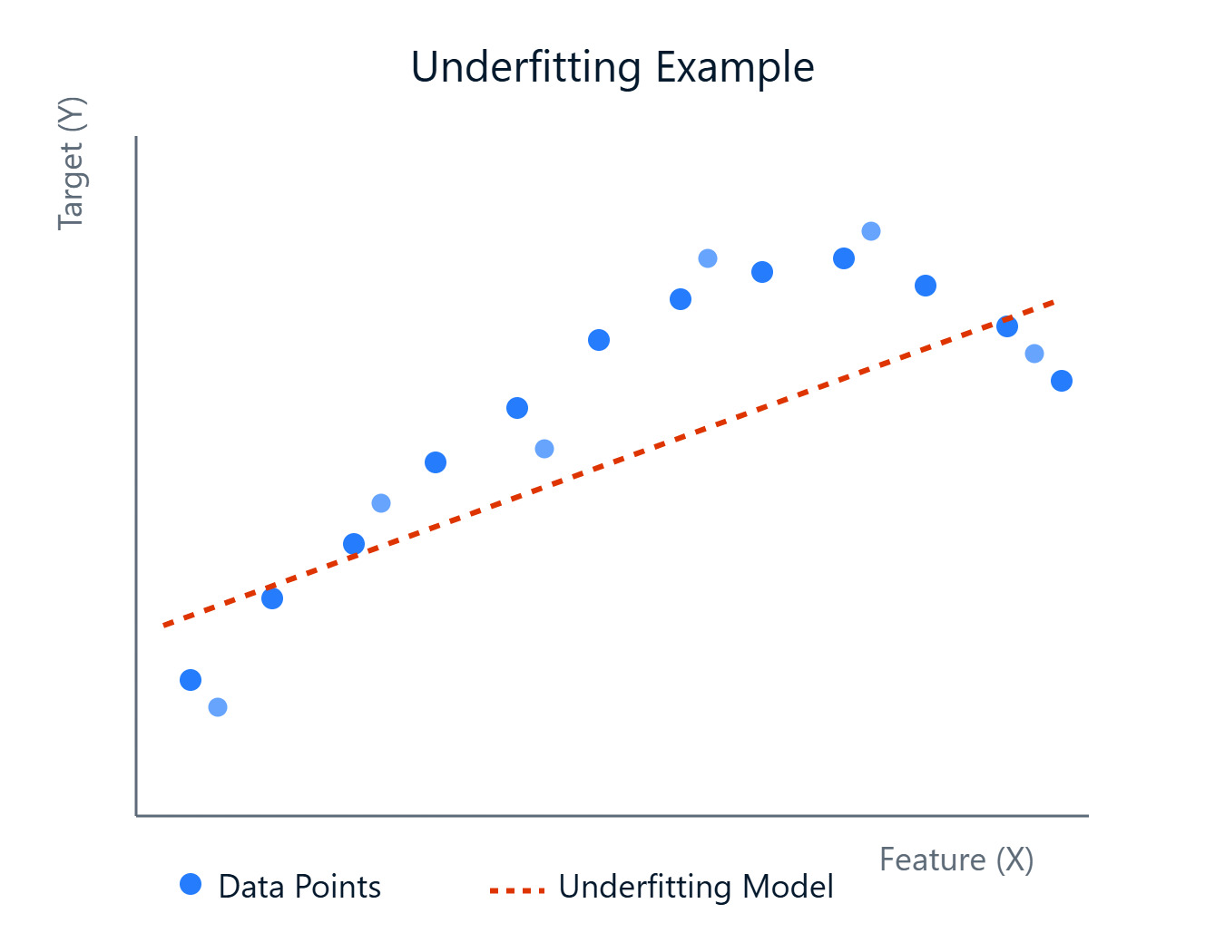
Image by Author

In this article, we'll take a look at what underfitting is, why it happens, how to spot it, and most importantly, how to fix underfitting. If you’re looking to get hands-on with machine learning, make sure to check out our Machine Learning Fundamentals in Python track. 

What is Underfitting?

Let's take a deeper look into the concept of underfitting and how it contrasts with its counterpart, overfitting. Understanding this distinction is fundamental to model diagnostics and improvement.

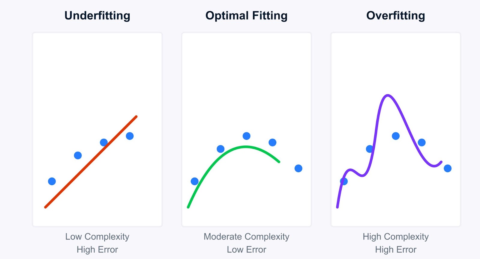
Image by Author

Simply put, Underfitting occurs when a machine learning model is too simple to capture the underlying patterns in the training data. Imagine trying to fit a straight line through data points that clearly follow a curve, and the line (our model) just isn't complex enough. An underfitting model suffers from high bias, meaning it makes strong assumptions about the data (e.g., assuming a linear relationship where there isn't one). 

Because it fails to learn the data well, it performs poorly not only on the training data but also on new, unseen data (test data). However, these models tend to have low variance, meaning their predictions don't change much if you train them on different subsets of the data. The simplicity makes them consistent, albeit consistently wrong.

Mathematically, this relates to the bias-variance decomposition of the model's expected error. The expected error of a model can be broken down into three components: bias squared, variance, and irreducible error:

Where:

• E[(y - f̂(x))²] is the expected squared error of the prediction.

• Bias(f̂(x)) measures the error introduced by approximating the real function f(x) with the model.

• Var(f̂(x)) is the variability of the model prediction for different training datasets.

• σ² represents the irreducible error — the inherent noise in the data that cannot be predicted.

In underfitting, theBias(f̂(x)) term dominates the error. The model is too simple, leading to systematic errors and a failure to capture the true data relationship.

Contrasting underfitting vs overfitting

Understanding underfitting becomes clearer when compared to overfitting. While underfitting models are too simple, overfitting models are too complex. They learn the training data too well, capturing not just the underlying patterns but also the noise and random fluctuations.

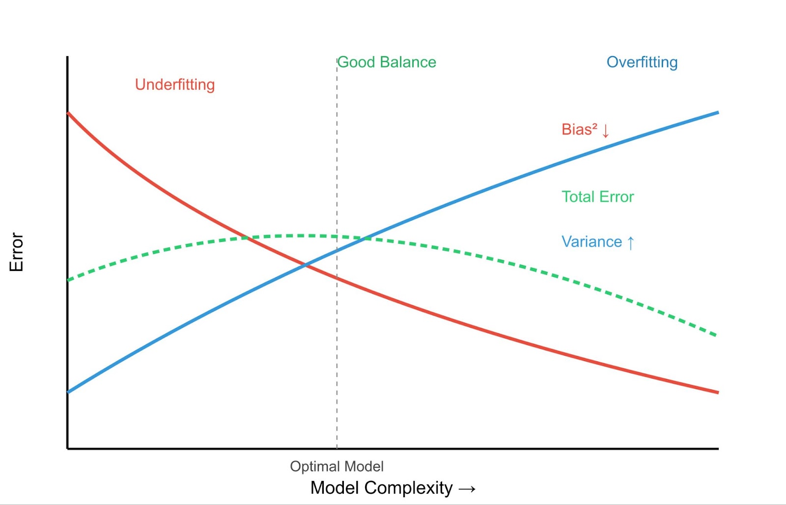
Bias Variance Trade-off - Image by Author

Let’s look at the key differences between Underfitting and Overfitting:

This leads to the crucial concept of the bias-variance trade-off.

• High Bias (Underfitting): Simple models have high bias but low variance. They are consistently wrong but don't vary much with different training data.
• High Variance (Overfitting): Complex models have low bias but high variance. They fit the training data very well (low bias) but are highly sensitive to the specific training data used, leading to poor generalization on new data. You can learn more about this in our article What is Overfitting?.

The goal is to find a sweet spot: a model complex enough to capture the true patterns (low bias) but not so complex that it learns the noise (low variance).

Examples:

• Underfitting Example: Trying to predict house prices, which depend on size, location, age, etc., using only the number of rooms. The model is too simple (high bias) and will likely make poor predictions for most houses.
• Overfitting Example: Creating a highly complex polynomial regression model that perfectly passes through every single data point in your house price training set. This model might have near-zero error on the training data, but it will perform terribly on new houses because it has learned the noise specific to the training set (high variance).

Understanding where your model falls on this spectrum is important for developing effective machine learning solutions, as we'll see in the following sections on detecting and addressing underfitting.

Causes of Underfitting and Diagnostic Indicators

Now that we understand what underfitting is, let's see why it happens and how you can detect it in your own projects. Identifying the root cause is essential for choosing the right mitigation strategy. 

Primary causes of underfitting

Several factors can lead to an underfitting model:

Insufficient model complexity

The chosen algorithm might be too simple for the data's underlying structure. For example, using a linear regression model when the relationship between features and the target variable is highly non-linear. The model inherently lacks the capacity to capture the complexities.

Inadequate training

The model might not have been trained for long enough (e.g., too few epochs in neural networks) or with appropriate learning parameters. If the training process stops prematurely, the model won't have had sufficient opportunity to learn the patterns, even if it has the capacity.

Poor feature representation 

The features used to train the model might not adequately represent the underlying factors influencing the target variable. This could mean:

• Missing important features: Key predictors weren't included in the dataset.
• Irrelevant features: The dataset contains noise or features that don't correlate with the outcome, potentially misleading a simple model.
• Features needing transformation: Features might require scaling, normalization, or encoding (e.g., categorical variables) to be useful for the model.

Excessive regularization

Regularization techniques (like L1 or L2 penalties) are primarily used to prevent overfitting by adding a penalty for complexity. However, if the regularization strength (e.g., the lambda parameter) is set too high, it can overly penalize the model, forcing it to become too simple and thus causing underfitting. Learn more about regularization in Towards Preventing Overfitting in Machine Learning: Regularization.

Low-quality or insufficient data

• Not enough data: If the training dataset is too small, the model may not have enough examples to learn the underlying patterns effectively.
• High noise: If the data is very noisy, the model might struggle to distinguish the signal from the noise, especially if it's a simple model.
• Missing values: Significant amounts of missing data can hinder the model's ability to learn, particularly if not handled properly. Techniques for dealing with this are covered in Handling Missing Data with Imputations in R.

Detection methods

How can you tell if your model is underfitting? Here are some common diagnostic techniques:

Analyzing performance metrics 

The most straightforward indicator is poor performance on both the training set and the validation/test set. If your model achieves high error (or low accuracy, low R-squared, etc.) on the data it was trained on, it's a strong sign it hasn't learned the patterns effectively. Unlike overfitting, where training performance is excellent, but test performance is poor, underfitting shows poor performance across the board.

Learning curves

Plotting the model's performance (e.g., error or accuracy) on the training and validation sets as a function of training time or dataset size can be very insightful. For an underfitting model, the learning curves typically show:

• High training error that plateaus early.
• High validation error that is close to the training error and also plateaus.
• Both curves converge at a high error level, indicating the model isn't improving significantly even with more data or training.

Feature analysis

Review the features used. Are they relevant? Are there interactions you haven't captured? Are numerical features scaled? Are categorical features encoded appropriately? 

Sometimes, revisiting feature engineering can reveal why the model is struggling. Basic concepts are covered in Machine Learning Fundamentals in R. For deeper insights into statistical relationships, consider resources like Statistical Inference in R.

Comparative modeling

Train a more complex model (e.g., a decision tree or gradient boosting machine if you initially used linear regression) on the same data. If the more complex model significantly outperforms your initial model on both training and validation sets, it suggests your original model was likely underfitting due to insufficient complexity. 

You can track such comparisons using the tools discussed in Machine Learning Experimentation: An Introduction to Weights & Biases.

By understanding these causes and detection methods, you can effectively diagnose an underfitting model and take steps to improve its performance.

Underfitting Mitigation Strategies and Best Practices

Once you've identified underfitting, the next step is knowing how to fix underfitting. Fortunately, several effective strategies can help increase your model's ability to learn the underlying patterns in the data. Let’s look at some of them:

Enhancing model complexity

If your model is too simple (high bias), making it more complex can often resolve underfitting. We can do that using the following ways:

Algorithm selection

Switch to a more powerful model. If linear regression is underfitting, try polynomial regression, decision trees, random forests, gradient boosting machines (like XGBoost or LightGBM), or support vector machines (SVMs) with non-linear kernels. These models inherently have more capacity to capture complex relationships.

Polynomial feature expansion

For regression problems, you can create polynomial features from your existing numerical features. This allows linear models to fit more complex, curved relationships. For example, if you have a feature x, you can add x2, x3, etc., as new features. Scikit-learn provides PolynomialFeatures for this.

Hyperparameter tuning

Many complex models have hyperparameters that control their complexity (e.g., the depth of a decision tree, the number of neurons in a neural network layer, the C parameter in SVMs). Tuning these hyperparameters to allow for more complexity can reduce bias. 

Techniques like Grid Search or Randomized Search are essential here. Learn more with courses like Hyperparameter Tuning in Python or Hyperparameter Tuning in R. See also our tutorial on Hyperparameter Optimization in Machine Learning Models.

Feature engineering and data augmentation

Sometimes, the model isn't the problem, it's the data representation. Improving the features can significantly help. We can do that in the following ways:

Domain-specific feature creation

Use your knowledge of the problem domain to create new features that might be more informative. For example, in predicting house prices, combining 'number of bedrooms' and 'number of bathrooms' into a 'total rooms' feature, or calculating 'house age' from 'year built'.

Interaction features

Create features that represent the interaction between existing features (e.g., multiplying two features together). This can help models capture synergistic effects.

Data enrichment

Augment your dataset with external data sources if possible. For example, adding demographic data to customer information or weather data to sales predictions.

Data augmentation (primarily for unstructured data)

For image or text data, techniques like rotating/flipping images or using synonym replacement in text can artificially increase the size and diversity of the training set, potentially helping the model learn more robust patterns.

Regularization adjustment

If underfitting is caused by excessive regularization intended to prevent overfitting, you need to dial it back. Lower the value of the regularization parameter (e.g., alpha in Ridge/Lasso, C in SVMs – note that for SVMs, a smaller C means stronger regularization, so you'd increase C).

If using dropout, reduce the dropout rate (the fraction of neurons dropped during training). A lower rate retains more network capacity.

Finding the right balance often requires careful tuning, again highlighting the importance of hyperparameter optimization.

Ensemble methods

Ensemble methods combine predictions from multiple individual models (weak learners) to produce a stronger, more robust final prediction. They are often very effective at reducing both bias and variance. Some of the ensemble methods are as follows:

• Bagging (e.g., Random Forests): Trains multiple models (e.g., decision trees) independently on different bootstrap samples of the data and averages their predictions. This primarily reduces variance but can also help if the base learners are slightly biased. Check out our Bagging tutorial for more info.
• Boosting (e.g., AdaBoost, Gradient Boosting): Trains models sequentially, with each new model focusing on correcting the errors made by the previous ones. Boosting is particularly effective at reducing bias and turning weak learners into strong ones, making it a powerful tool against underfitting. We have a . Boosting guide to explain more. 
• Stacking: Trains multiple different types of models and then uses another model (a meta-learner) to learn how to best combine their predictions.

By applying these strategies, often in combination, you can effectively address underfitting and build models that better capture the complexities of your data.

Practical Applications and Case Studies

Seeing underfitting in action with datasets and code can significantly clarify the concept. Let’s look at practical examples to demonstrate how an underfitting model behaves and how its performance can be improved.

Linear regression underfitting example

A common scenario for underfitting occurs when a simple linear model is used to describe a non-linear relationship. Let's illustrate this by attempting to fit a linear regression model to data that follows a quadratic pattern.

We will generate synthetic data where the target variable y has a quadratic relationship with a feature X. First, we'll fit a simple linear regression model. We'll observe its poor performance (high Mean Squared Error - MSE) and visualize how it fails to capture the data's curve. 

Then, we'll expand the features by adding a polynomial term and fit a polynomial regression model. This will demonstrate how increasing model complexity can reduce bias and significantly improve the model's accuracy.

Let’s start by importing the necessary libraries as follows:

# Import necessary libraries
import numpy as np
import matplotlib.pyplot as plt
from sklearn.linear_model import LinearRegression
from sklearn.preprocessing import PolynomialFeatures
from sklearn.pipeline import make_pipeline
from sklearn.metrics import mean_squared_error

Let’s generate synthetic non-linear data . We'll create data with a quadratic relationship: y = 0.5*X^2 + X + 2 + noise.

np.random.seed(42) # for reproducibility
num_samples = 100
X = np.sort(10 * np.random.rand(num_samples, 1) - 5, axis=0) # Feature X (sorted for plotting)
y_true = 0.5 * X**2 + X + 2 # True quadratic relationship
y = y_true + np.random.randn(num_samples, 1) * 5 # Add some noise to make it realistic

Now, we’ll fit a simple linear regression model (Underfitting Model) as shown below:

linear_model = LinearRegression()
linear_model.fit(X, y)
y_pred_linear = linear_model.predict(X)
mse_linear = mean_squared_error(y, y_pred_linear)

print(f"--- Simple Linear Regression (Potential Underfitting Model) ---")
print(f"Mean Squared Error (MSE): {mse_linear:.2f}")
print(f"Model Coefficients (slope): {linear_model.coef_[0][0]:.2f}")
print(f"Model Intercept: {linear_model.intercept_[0]:.2f}")

Output:

--- Simple Linear Regression (Potential Underfitting Model) ---

Mean Squared Error (MSE): 34.03

Model Coefficients (slope): 1.00

Model Intercept: 6.42

Now, we’ll fit a polynomial regression model (Improved Model). To do that, we create polynomial features (degree 2) and then fit a linear model to these features. The PolynomialFeatures step adds new features. The LinearRegression step has coefficients for each.

For degree 2, we expect coefficients for X and X^2. A pipeline makes this process cleaner. The named_steps attribute of the pipeline allows access to individual steps as shown below:

polynomial_model = make_pipeline(PolynomialFeatures(degree=2, include_bias=False), LinearRegression())
polynomial_model.fit(X, y)
y_pred_poly = polynomial_model.predict(X)
mse_poly = mean_squared_error(y, y_pred_poly)

print(f"\n--- Polynomial Regression (Degree 2) ---")
print(f"Mean Squared Error (MSE): {mse_poly:.2f}")
poly_reg_coeffs = polynomial_model.named_steps['linearregression'].coef_[0]
poly_reg_intercept = polynomial_model.named_steps['linearregression'].intercept_[0]
print(f"Model Coefficients (for X, X^2): {poly_reg_coeffs[0]:.2f}, {poly_reg_coeffs[1]:.2f}")
print(f"Model Intercept: {poly_reg_intercept:.2f}")

Output:

--- Polynomial Regression (Degree 2) ---

Mean Squared Error (MSE): 20.48

Model Coefficients (for X, X^2): 1.13, 0.50

Model Intercept: 2.04

Now let’s visualize the model fitting as showb below:

# Visualization
plt.figure(figsize=(10, 4))
plt.scatter(X, y, s=30, label="Actual Data Points", alpha=0.7, edgecolors='k')
plt.plot(X, y_pred_linear, color='red', linewidth=2, label=f'Linear Fit (Underfitting)\nMSE: {mse_linear:.2f}')
plt.plot(X, y_pred_poly, color='green', linewidth=2, label=f'Polynomial Fit (Degree 2)\nMSE: {mse_poly:.2f}')
plt.title('Demonstrating Underfitting with Linear vs. Polynomial Regression', fontsize=16)
plt.xlabel('Feature X', fontsize=14)
plt.ylabel('Target y', fontsize=14)
plt.legend(fontsize=12)
plt.grid(True, linestyle='--', alpha=0.7)
plt.show()

Output:

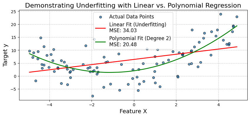
The plot visually confirms the underfitting of the simple linear model. It fails to capture the curve in the data. The polynomial regression model, by incorporating the X^2 term, provides a much better fit, as evidenced by its lower MSE.

This shows how expanding features (increasing model complexity) can reduce bias and improve accuracy when the underlying relationship is non-linear. Next, let’s look at a medical diagnosis case study.

Medical diagnosis case study

Let's simulate a medical diagnosis scenario using the well-known Breast Cancer Wisconsin (Diagnostic) dataset available in scikit-learn.

We'll first attempt to build a classification model using only a very limited subset of features, which might lead to underfitting. Then, we'll use a more comprehensive set of features and potentially a more complex algorithm to demonstrate improvement.

Let’s start by importing the necessary libraries as follows:

# Import necessary libraries
import numpy as np
import pandas as pd
import matplotlib.pyplot as plt
from sklearn.datasets import load_breast_cancer
from sklearn.model_selection import train_test_split
from sklearn.preprocessing import StandardScaler
from sklearn.linear_model import LogisticRegression
from sklearn.ensemble import RandomForestClassifier
from sklearn.metrics import accuracy_score, roc_auc_score, confusion_matrix, ConfusionMatrixDisplay

Now, let’s load and prepare the data:

cancer = load_breast_cancer()
X = pd.DataFrame(cancer.data, columns=cancer.feature_names)
y = cancer.target # 0 for malignant, 1 for benign

For demonstration, let's select a very limited subset of features for the underfitting scenario. These might not be the most predictive on their own:

features_limited = ['mean texture', 'mean symmetry']
X_limited = X[features_limited]

For the improved model, we'll use a larger subset (or all features). Let's pick the first 10 features for a more comprehensive set:

features_comprehensive = cancer.feature_names[:10]
X_comprehensive = X[features_comprehensive]

Let’s split data. We'll do this separately for each feature set for clarity:

X_train_lim, X_test_lim, y_train, y_test = train_test_split(X_limited, y, test_size=0.3, random_state=42, stratify=y)
X_train_comp, X_test_comp, _, _ = train_test_split(X_comprehensive, y, test_size=0.3, random_state=42, stratify=y) # y_train and y_test are the same

Let’s scale features as this is important for logistic regression and many other algorithms:

scaler_lim = StandardScaler().fit(X_train_lim)
X_train_lim_scaled = scaler_lim.transform(X_train_lim)
X_test_lim_scaled = scaler_lim.transform(X_test_lim)

scaler_comp = StandardScaler().fit(X_train_comp)
X_train_comp_scaled = scaler_comp.transform(X_train_comp)
X_test_comp_scaled = scaler_comp.transform(X_test_comp)

Now, let’s fit a logistic regression with limited features:

print("Scenario 1: Logistic Regression (Limited Features - Potential Underfitting)")
log_reg_limited = LogisticRegression(random_state=42, solver='liblinear') # liblinear is good for small datasets
log_reg_limited.fit(X_train_lim_scaled, y_train)
y_pred_lim = log_reg_limited.predict(X_test_lim_scaled)
y_proba_lim = log_reg_limited.predict_proba(X_test_lim_scaled)[:, 1]

acc_lim = accuracy_score(y_test, y_pred_lim)
auc_lim = roc_auc_score(y_test, y_proba_lim)
print(f"Features used: {features_limited}")
print(f"Accuracy: {acc_lim:.4f}")
print(f"AUC: {auc_lim:.4f}")

Output:

Scenario 1: Logistic Regression (Limited Features - Potential Underfitting)

Features used: ['mean texture', 'mean symmetry']

Accuracy: 0.7544

AUC: 0.8151

Let’s adopt a mitigation strategy. We’ll fit a logistic regression model with more features:

print("Scenario 2: Logistic Regression (Comprehensive Features)")
log_reg_comp = LogisticRegression(random_state=42, solver='liblinear')
log_reg_comp.fit(X_train_comp_scaled, y_train)
y_pred_comp_lr = log_reg_comp.predict(X_test_comp_scaled)
y_proba_comp_lr = log_reg_comp.predict_proba(X_test_comp_scaled)[:, 1]

acc_comp_lr = accuracy_score(y_test, y_pred_comp_lr)
auc_comp_lr = roc_auc_score(y_test, y_proba_comp_lr)
print(f"Features used: First 10 features") # For brevity
print(f"Accuracy: {acc_comp_lr:.4f}")
print(f"AUC: {auc_comp_lr:.4f}")

Output:

Scenario 2: Logistic Regression (Comprehensive Features)

Features used: First 10 features

Accuracy: 0.9181

AUC: 0.9831

Now, let’s fit a more complex model like Random Forest with more features:

print("Scenario 3: Random Forest (Comprehensive Features)")
rf_comp = RandomForestClassifier(random_state=42, n_estimators=100) # n_estimators is a key hyperparameter
rf_comp.fit(X_train_comp_scaled, y_train) # RF can also benefit from scaled data, though less sensitive
y_pred_comp_rf = rf_comp.predict(X_test_comp_scaled)
y_proba_comp_rf = rf_comp.predict_proba(X_test_comp_scaled)[:, 1]

acc_comp_rf = accuracy_score(y_test, y_pred_comp_rf)
auc_comp_rf = roc_auc_score(y_test, y_proba_comp_rf)
print(f"Features used: First 10 features")
print(f"Accuracy: {acc_comp_rf:.4f}")
print(f"AUC: {auc_comp_rf:.4f}")

Output:

Scenario 3: Random Forest (Comprehensive Features)

Features used: First 10 features

Accuracy: 0.9415

AUC: 0.9878

Let’s plot and compare the confusion matrix for each case:

fig, axes = plt.subplots(1, 3, figsize=(20, 5))
fig.suptitle('Comparison of Model Performance (Confusion Matrices on Test Set)', fontsize=16)

# Model 1: Logistic Regression (Limited Features)
cm_lim = confusion_matrix(y_test, y_pred_lim)
disp_lim = ConfusionMatrixDisplay(confusion_matrix=cm_lim, display_labels=cancer.target_names)
disp_lim.plot(ax=axes[0], cmap='Blues')
axes[0].set_title(f'LogReg (Limited Features)\nAcc: {acc_lim:.2f}, AUC: {auc_lim:.2f}')

# Model 2: Logistic Regression (Comprehensive Features)
cm_comp_lr = confusion_matrix(y_test, y_pred_comp_lr)
disp_comp_lr = ConfusionMatrixDisplay(confusion_matrix=cm_comp_lr, display_labels=cancer.target_names)
disp_comp_lr.plot(ax=axes[1], cmap='Greens')
axes[1].set_title(f'LogReg (Comprehensive Features)\nAcc: {acc_comp_lr:.2f}, AUC: {auc_comp_lr:.2f}')

# Model 3: Random Forest (Comprehensive Features)
cm_comp_rf = confusion_matrix(y_test, y_pred_comp_rf)
disp_comp_rf = ConfusionMatrixDisplay(confusion_matrix=cm_comp_rf, display_labels=cancer.target_names)
disp_comp_rf.plot(ax=axes[2], cmap='Oranges')
axes[2].set_title(f'Random Forest (Comprehensive Features)\nAcc: {acc_comp_rf:.2f}, AUC: {auc_comp_rf:.2f}')

plt.tight_layout(rect=[0, 0, 1, 0.96]) # Adjust layout to make space for suptitle
plt.show()

Output:

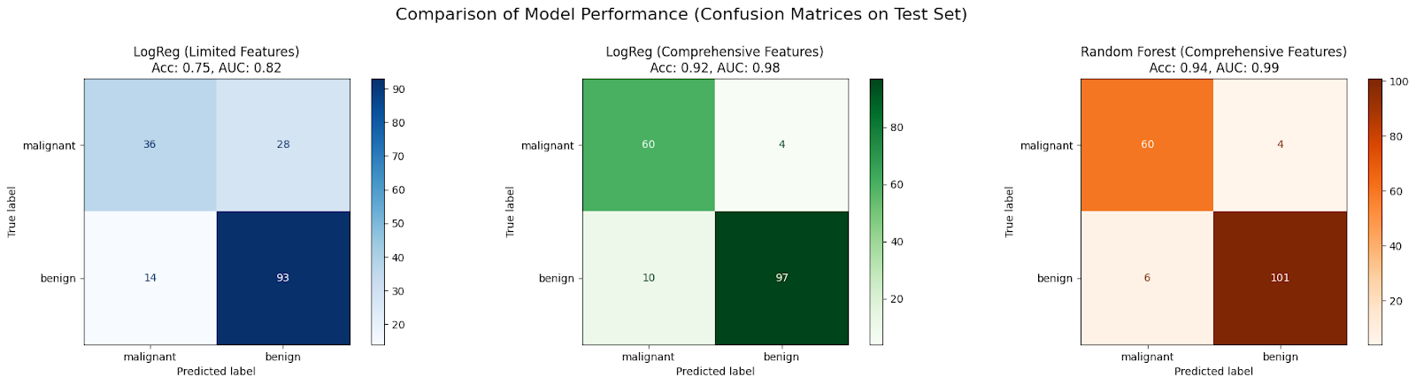
In this case study, an initial LogisticRegression model trained on only two features (Scenario 1) is expected to underfit due to insufficient information, resulting in poor accuracy and AUC. 

Performance typically improved when the same algorithm is given a more comprehensive set of features (Scenario 2), as it has more data to learn from, reducing bias.

Further improvement is often seen by using a more complex algorithm like RandomForestClassifier with the comprehensive feature set (Scenario 3), because it can capture non-linearities and feature interactions more effectively, further reducing bias and enhancing the model's fit to the data.

Advanced Topics and Future Directions

While we've covered the fundamentals, the landscape of machine learning is always evolving. Here's a brief look at how underfitting relates to more advanced areas.

The role of deep learning

Deep learning models, particularly deep neural networks with many layers, are known for their high capacity, meaning they can theoretically approximate very complex functions.

Due to their inherent complexity, deep learning models are generally less prone to underfitting than simpler models, provided they are trained properly on sufficient data. Their structure allows them to automatically learn intricate feature representations from raw data (like pixels in images or words in text).

However, deep learning isn't immune to issues that look like underfitting. If a network is poorly designed (e.g., insufficient depth/width for the task), not trained long enough, or uses inappropriate activation functions or optimization algorithms, it might still fail to converge and exhibit high training error.

Architectural innovations like residual connections (ResNets) and normalization techniques (Batch Normalization) help train very deep networks effectively, mitigating vanishing/exploding gradient problems and enabling them to reach their full capacity, thus avoiding convergence issues that mimic underfitting.

Automated machine learning (AutoML)

Finding the right model, features, and hyperparameters to avoid both underfitting and overfitting can be time-consuming. AutoML aims to automate this process.

AutoML frameworks can automatically explore different model types (from linear models to complex ensembles and neural networks), perform feature engineering and selection, and optimize hyperparameters. By systematically searching a vast space of possibilities, AutoML can identify model configurations that have sufficient complexity to avoid underfitting the data.

Methods like Neural Architecture Search (NAS) automatically design network architectures, while sophisticated hyperparameter optimization techniques (e.g., Bayesian Optimization) efficiently find good hyperparameter settings. These tools can significantly accelerate the process of finding a well-fitting model, reducing the manual effort needed to diagnose and fix an underfitting model.

Conclusion

Understanding the underfitting vs overfitting dilemma is fundamental to successful machine learning. We've seen that underfitting arises when a model is too simple (high bias) to capture the underlying trends in the data, leading to poor performance on both training and unseen data. Key causes include insufficient model complexity, poor features, inadequate training, and excessive regularization.

Diagnosing underfitting involves examining performance metrics, plotting learning curves, and comparing models, often aided by code. Fortunately, we have several strategies for how to fix underfitting: increasing model complexity (choosing better algorithms, feature expansion, hyperparameter tuning), improving features (feature engineering, data enrichment), adjusting regularization, and employing powerful ensemble methods, as demonstrated in our code examples.

To learn about these techniques and more with hands-on examples, check out our Machine Learning Fundamentals in Python skill track.