How to Alternate Row Colors in Excel: A Helpful Guide

You can alternate row colors in Excel by using table styles or conditional formatting. These methods apply banded rows (rows formatted with alternating background colors) that make your data easier to read and scan.

When you work with large datasets, rows can blend. This slows you down and increases the chance of reading the wrong values. Alternating row colors creates visual separation between rows, which improves clarity and accuracy.

In this guide, you will learn step by step how to apply alternating row colors using Excel tables and conditional formatting. You will also see when to use each method based on your data and formatting needs.

How to Alternate Row Colors in Excel Using Tables

To alternate row colors using Excel tables, follow this step by step approach: 

Step 1: Convert the range into a table

To convert the range into a table: 

1. Click anywhere inside your data range

2. Press Ctrl + T on Windows or Command + T on Mac. You can also go to the Insert tab and click Table

3. The Create Table dialog box will appear. Excel selects your data automatically. Confirm that the range is correct

4. Select My table has headers if your first row contains column names

5. Click OK

Excel converts your range into a table and applies alternating row colors by default. Now the default table style includes:

• A bold header row
• Alternating background colors for rows
• Filter arrows in each column

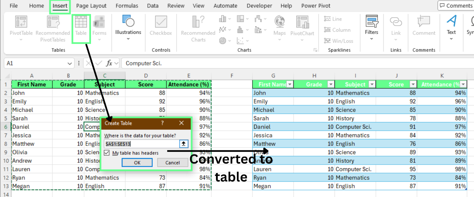
Convert the range into an Excel table. Image by Author.

Step 2: Change the alternating row colors

To change the default colors:  

1. Click anywhere inside the table
2. Go to the Table Design tab in the ribbon (or Table Tools > Design)
3. Locate the Table Styles section
4. Click the arrow to open the full style gallery
5. Select a style you prefer

Excel updates the alternating row colors instantly. Each style uses a different color pattern.

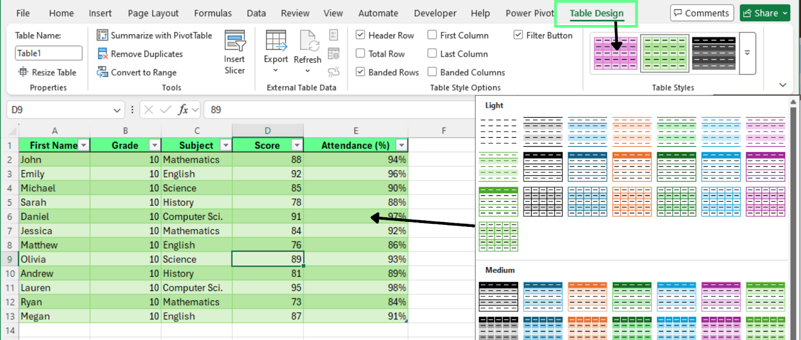
Choose a different alternate style color for your table. Image by Author.

To control the banded effect:

1. Go to Table Design
2. Use the Banded Rows checkbox under Table Style Options

When you enable Banded Rows, Excel displays alternating colors. When you clear it, Excel applies one background color to all rows.

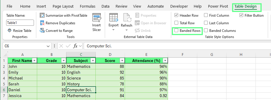
Disabling Banded Rows to apply the same background color. Image by Author.

Step 3: See how tables adjust automatically

Tables maintain the alternating pattern automatically. To see this:

1. Click in the last row of the table
2. Press Tab

Excel adds a new row and applies the correct alternating color. The pattern updates instantly when you delete rows as well. This keeps your spreadsheet consistent.

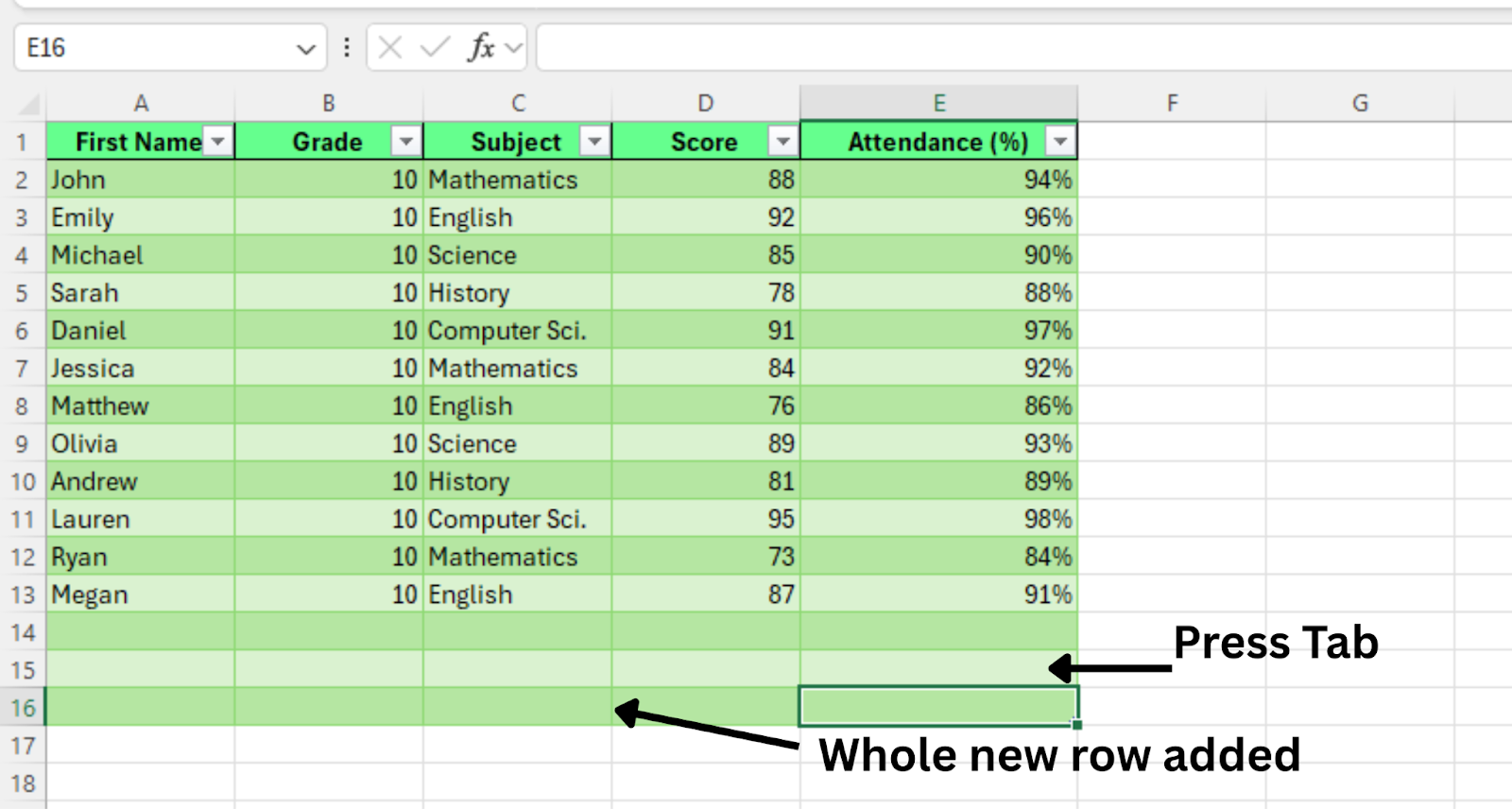
New row added. Image by Author.

If you want to convert the table back to a normal range while keeping the banded colors:

1. Click inside the table
2. Go to Table Design
3. Click Convert to Range

Excel removes the table structure. The Table Design tab disappears from the ribbon. The alternating row colors remain in place.

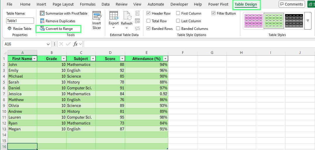
Convert the table to the normal range. Image by Author.

Converting your data into an Excel table is the fastest and most reliable way to apply alternating row colors.

Excel tables automatically apply banded rows (alternating background colors such as white and light gray). The formatting also updates when you add or remove data. This makes tables ideal for beginners and for datasets that change often.

How to Alternate Row Colors in Excel Using Conditional Formatting

To alternate row colors using conditional formatting:

• Select the data range where you want alternating colors. Leave out the header row

• Go to the Home tab

• Click Conditional Formatting > New Rule

• Select Use a formula to determine which cells to format

• Enter this formula: =MOD(ROW(),2)=0

Here is how the formula works:

• ROW() returns the current row number

• MOD(number,2) divides the row number by 2 and returns the remainder

• =0 applies formatting to even-numbered rows

• Use =1 if you want to format odd-numbered rows instead

Next:

• Click Format
• Open the Fill tab
• Choose the color you want for the alternating rows
• Click OK, then click OK again to apply the rule

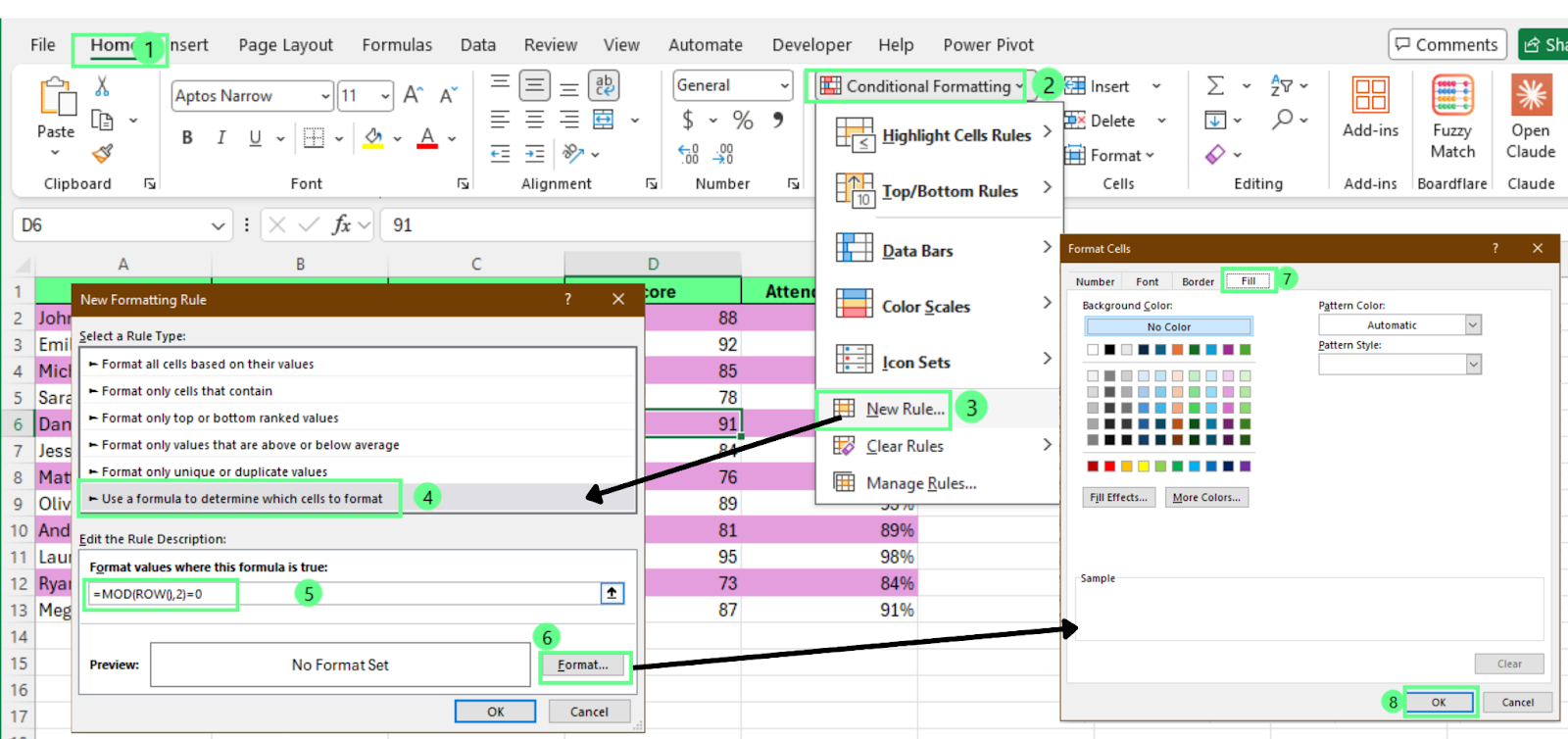
Apply Conditional Formatting to color the alternative row. Image by Author.

You can now see Excel applies the selected color to every second row within the chosen range.

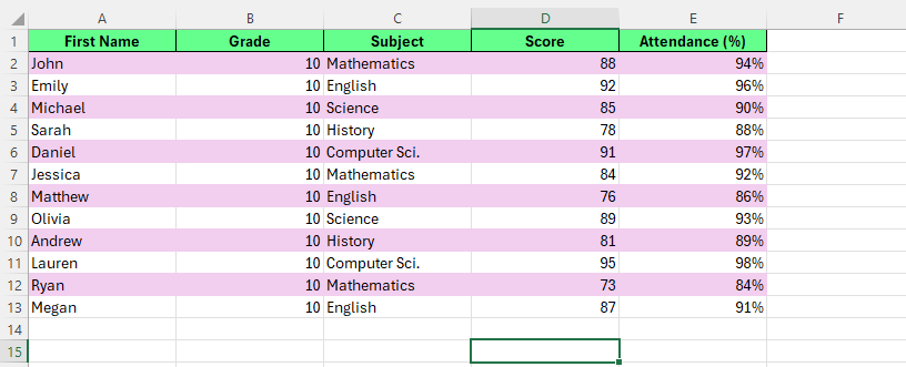
Color alternate rows using Conditional Formatting. Image by Author.

Use conditional formatting when you want full control over which rows Excel colors and how the pattern appears. This method works well when your data is in a normal range instead of a table, or when you want a custom rule for alternating rows.

Note: Conditional formatting applies only to the selected range. New rows added outside the range will not inherit the formatting automatically.

How to Alternate Row Colors in Excel Starting from a Specific Row

To alternate row colors in Excel starting from a specific row, follow the same steps you used for conditional formatting. Only change the formula.

Use this formula:

=MOD(ROW()-1,2)=0

Here is how it works:

• ROW() returns the current row number

• Subtracting 1 shifts the alternating pattern down by one row

• MOD(number,2) checks whether the row number is even or odd

• =0 applies the color to even rows. Use =1 to color odd rows instead

Change the number you subtract based on where your data starts.

For example:

• If your data starts on row 2, subtract 1

• If your data starts on row 3, subtract 2

• If your data starts on row 5, subtract 4

Match the subtraction value to one row above your first data row. This keeps the alternating pattern aligned with your dataset.

How to Alternate Row Colors in Excel Using VBA

To alternate colors in Excel using VBA, follow these steps:

Step 1: Save the workbook as a macro-enabled file

Before you start, save your workbook as an .xlsm file:

1. Click File
2. Select Save As
3. Choose Excel Macro Enabled Workbook (.xlsm)

Step 2: Open the VBA editor

To open VBA editor:

1. Select the data range you want to shade

2. Press Alt + F11 to open the VBA editor

3. Click Insert > Module

Step 3: Paste the VBA code

Paste this code into the Module window:

Sub BandRows()
   Dim rng As Range
   Dim r As Long
  
   If TypeName(Selection) <> "Range" Then Exit Sub
   Set rng = Selection
  
   'Clear existing fills in the selection
   rng.Interior.Pattern = xlNone
  
   'Start at row 2 of the selection to skip headers
   For r = 2 To rng.Rows.Count
       If (r Mod 2) = 0 Then
           rng.Rows(r).Interior.Color = RGB(255, 182, 193)
       End If
   Next r
End Sub

Step 4: Run the macro

You can run the macro in two ways:

• Click the green Run button in the VBA editor

• Or close the editor, press Alt + F8, select BandRows, and click Run

Excel colors every second row in the selected range. The macro skips the first row of the selection, which works well when the first row contains headers.

If you want to color the first data row instead, change this line:

If (r Mod 2) = 0 Then

to

If (r Mod 2) = 1 Then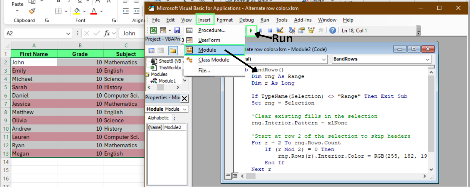

Color the alternate rows using the VBA editor. Image by Author.

This method applies colors once and keeps them static. Unlike tables or conditional formatting that work better for datasets that grow over time, it works well for final reports or files you plan to share. 

So, use VBA when:

• You want one-time formatting before sharing a file
• You need consistent styling across reports
• The dataset stays unchanged after formatting

How to Alternate Row Colors in Excel When the Data Changes

When your data changes, you can use either tables or conditional formatting to alternate row colors:

Using Excel tables for dynamic data

When you convert a range into a table, Excel manages the banded rows automatically.

Here is what happens:

• New rows receive the correct alternating color.
• Deleted rows adjust the pattern instantly.
• Sorting keeps the banding aligned with the data.
• Filtering preserves the visual structure.

Since tables handle frequent updates smoothly, they are the best option for dynamic datasets.

Using Conditional Formatting for changing data

Conditional formatting recalculates the formula whenever your data changes.

When you add, delete, or sort rows, Excel reevaluates the rule and reapplies the colors.

However, certain actions can affect the visual sequence:

• Hiding rows can shift the visible color pattern.
• Filtering may change how the banding appears on screen.
• Complex rules can reduce performance in large worksheets.

Conditional formatting works well for custom layouts and moderate edits. For ongoing data entry and frequent updates, tables offer a more consistent experience.

How to Alternate Column Colors Instead

To alternate column colors, you can either use table, conditional formatting, or VBA:

Using table

Excel tables include a built-in option for alternating columns. To enable it:

1. Click anywhere inside your table
2. Go to the Table Design tab
3. In the Table Style Options group, select Banded Columns

Excel applies alternating colors to columns instantly. But you can clear Banded Rows if you want only column shading.

The column pattern updates automatically when you add or remove columns.

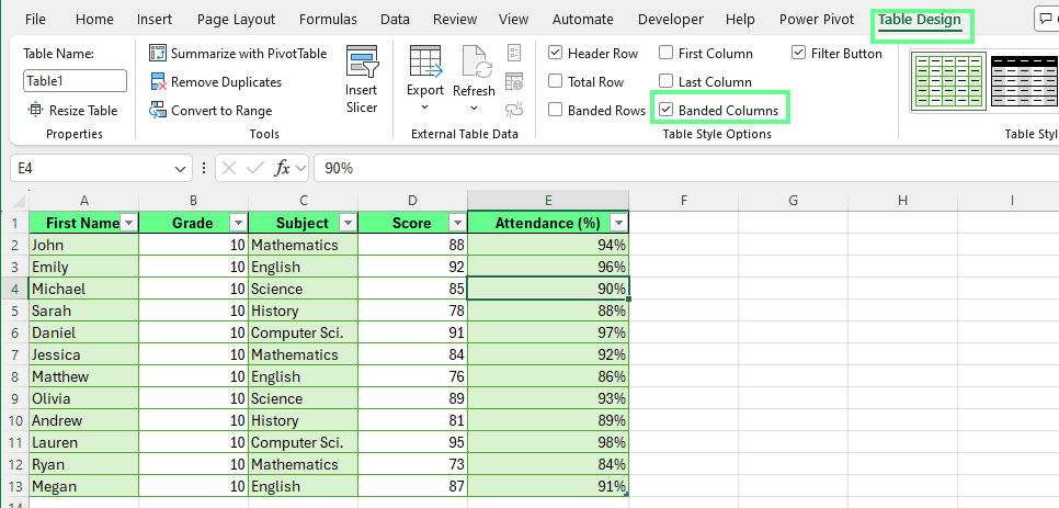
Alternate column color using the Banded Columns option. Image by Author. 

Using conditional formatting

To apply alternating column colors using conditional formatting:  

1. Select the data range where you want alternating column colors

2. Go to Home > Conditional Formatting > New Rule

3. Select Use a formula to determine which cells to format

4. Enter this formula: =MOD(COLUMN(),2)=0

Here is how it works:

• COLUMN() returns the current column number

• MOD(number,2) checks whether the column number is even or odd

• =0 applies formatting to even columns

• Use =1 to format odd columns instead

Next:

• Click Format > Fill tab
• Choose a color
• Click OK, then click OK again

Excel applies the selected color to every second column in the chosen range.

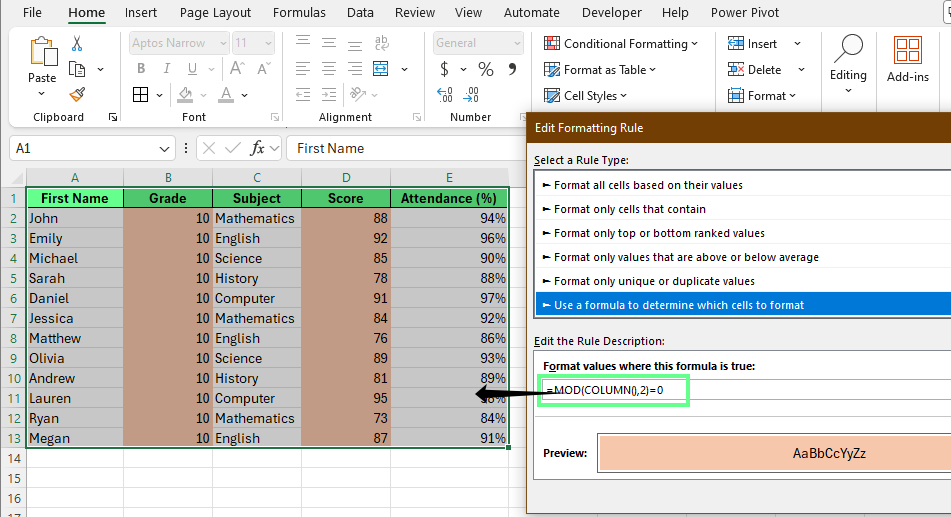
Color alternate columns using conditional formatting. Image by Author.

Using VBA

To apply column banding one time using VBA, open the VBA editor and paste this code into a new module:

Sub BandColumns()
   Dim rng As Range
   Dim c As Long

   If TypeName(Selection) <> "Range" Then Exit Sub
   Set rng = Selection

   'Clear existing fills
   rng.Interior.Pattern = xlNone

   'Start from column 2 to skip first column
   For c = 2 To rng.Columns.Count
       If (c Mod 2) = 0 Then
           rng.Columns(c).Interior.Color = RGB(255, 182, 193)
       End If
   Next c
End Sub

Run the macro to color every second column in the selected range. The code skips the first column, which works well when it contains labels.

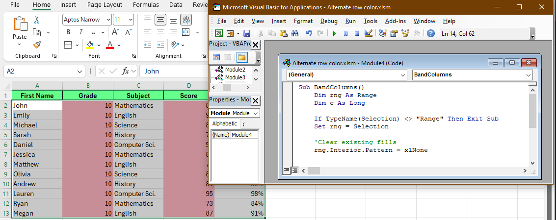
Color alternate columns using the VBA editor. Image by Author.

How to Remove Alternating Row Colors in Excel

To remove alternating row colors, you can use table settings, conditional formatting rules, or format clearing for VBA based shading — depending on your needs. 

Using table

To use table for removing colors: 

1. Select any cell inside the table
2. Go to the Table Design tab
3. In the Table Styles group, click the drop down arrow
4. Select Clear

You can also clear the checkboxes for Banded Rows and Banded Columns under Table Style Options. As a result, Excel removes the alternating colors and keeps the table structure intact.

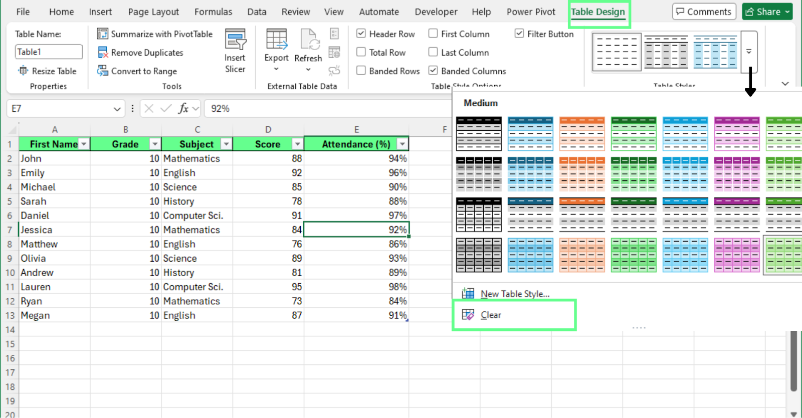
Clear the alternate color using table design option. Image by Author.

Using conditional formatting

If you applied alternating colors using conditional formatting, follow these steps to remove it:

1. Select the formatted range
2. Go to Home > Conditional Formatting > Manage Rules
3. Select the alternating row rule
4. Click Delete Rule
5. Click OK

Excel removes the color pattern from the selected range.

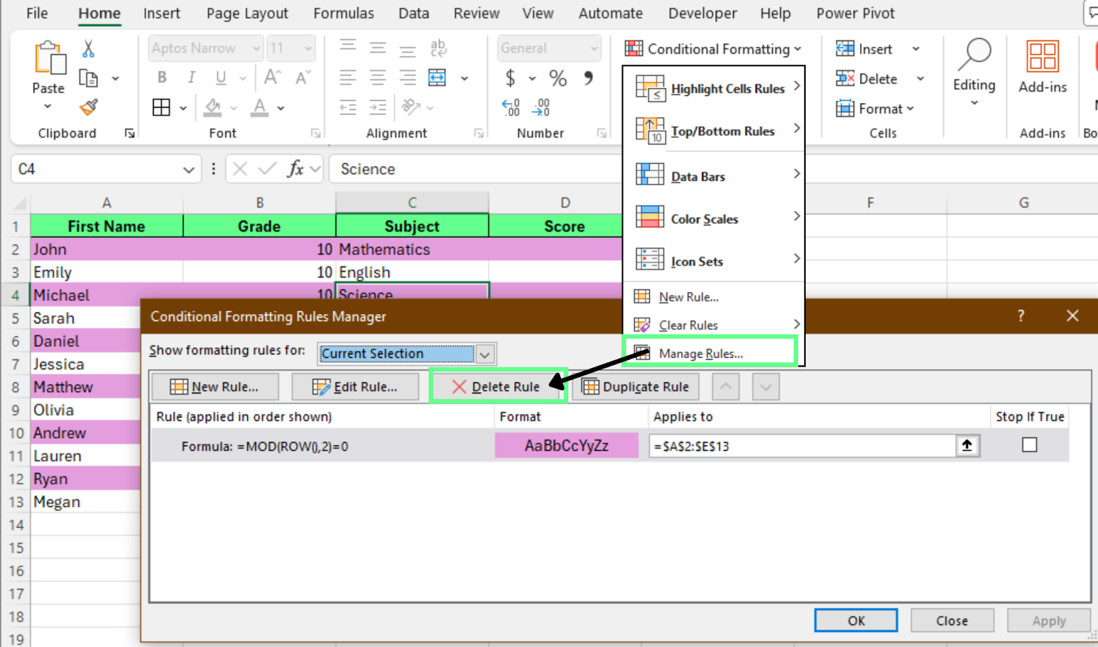
Clear conditional formatting alternate color. Image by Author.

Using VBA 

To remove colors that you applied using a macro: 

1. Select the affected cells
2. Go to Home > Clear > Clear Formats

Excel removes all formatting from the selected cells, including background colors. This action clears every format applied to those cells.

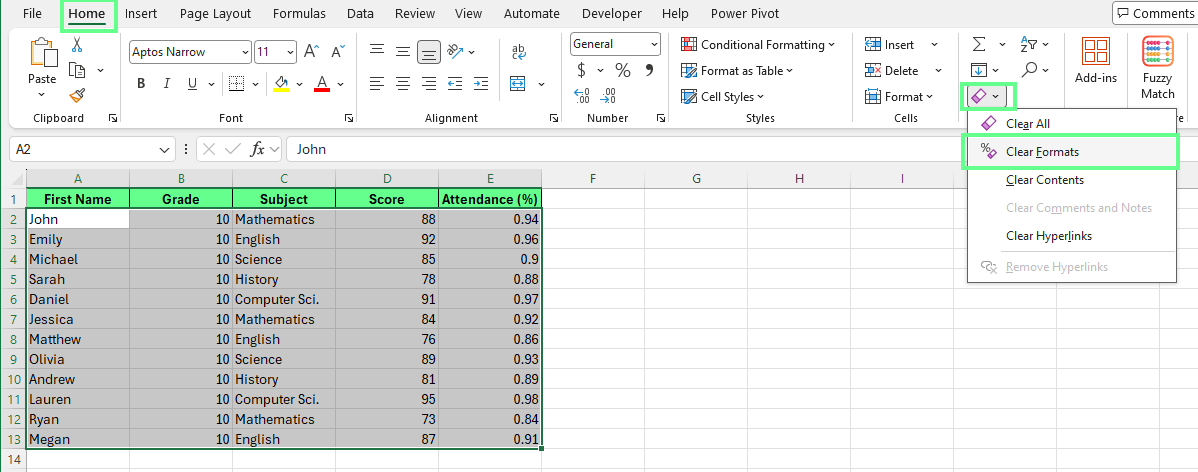
Remove the alternate color using the Clear Formats button. Image by Author.

After removing banding

Review your worksheet after removing alternating colors. Check that:

• Headers remain clear and distinct
• Columns stay easy to scan
• Important values still stand out

Clean formatting keeps your data readable, even without color banding.

Best Practices for Alternating Row Colors in Excel

Alternating row colors improve readability, but the way you apply them is important. In our experience, a few simple habits keep your worksheet clean, consistent, and easy to maintain.

We recommend the following best practices:

• Use tables whenever possible: Tables apply alternating row colors automatically and keep the pattern consistent as data changes.
• Use conditional formatting for custom layouts: This method gives you more control when a table does not match your structure.
• Choose subtle colors: Light shades help readers follow rows without drawing attention away from the data.
• Limit extra formatting in large datasets: Excess styling affects performance and makes worksheets harder to scan.
• Maintain consistency across reports: A uniform banding style makes data easier to compare and review.

Final Thoughts

Now that you know how to alternate row colors in Excel, apply the method that fits your workflow: 

• Use tables for dynamic datasets
• Use conditional formatting when you need precise control
• Keep your formatting simple and consistent so your data stays easy to scan as it grows

As a next step, strengthen your worksheet structure. Clean your data, remove blank rows, and organize columns before applying visual styling. You can also explore DataCamp’s guide on Highlight duplicates in Excel to add another layer of clarity to your analysis and make your spreadsheets easier to review.