Feed-Forward Neural Networks Explained: A Complete Tutorial

When looking at Machine Learning Algorithms, there are very few concepts as fundamental as the Feed-Forward Neural Network (FFNN). If you have ever built your first neural network, there's a good chance it was a feed-forward one. They can be seen almost everywhere - from simple classification problems to powering layers in deep architectures. 

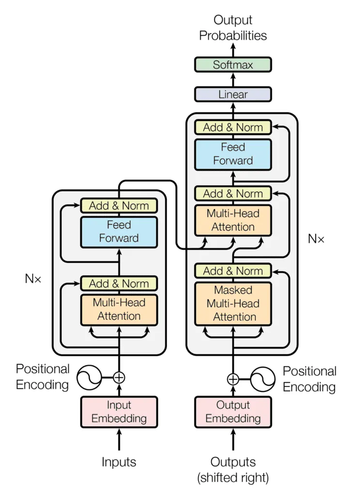
Let me first show you where Feed-Forward Neural Networks come in the broad scheme of things:

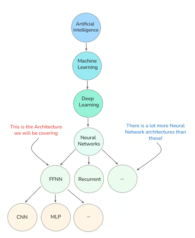
In this tutorial, I will explain what a Feed-Forward Neural Network actually is, how it evolved, and why it is still relevant today, as well as explore real-world examples.

What is a Feed-Forward Neural Network?

Intuitively speaking, the best way to describe such a network architecture is “Data flows only forward, no loops.”

At its core, a FFNN processes data in such a way that it flows in one direction, from input to output. There is no looping back, no recursion, and no cycles (excluding backpropagation, which we will get to shortly). 

When I was first learning about this, the mental image that helped me most was a factory conveyor belt. 

Why? 

Because each step in the process (or each layer in the network) does something simple to the input before passing it along to the next.

Here's how it works:

1. Inputs go into the first layer (the input layer).
2. They're transformed by weights and biases and passed through an activation function.
3. This continues through one or more hidden layers.
4. Finally, the output layer makes a prediction.

Before I show you what such a network architecture looks like, I want to clear a common misconception:

“Feed-Forward Neural Networks are the same as MLPs.”

To clear this misconception, we need to explore the early history of Deep Learning. 

Early history of deep learning

Perceptron: We start with the Perceptron, which was invented in the 1950s by Frank Rosenblatt. It was a single-layer binary classifier, and while it couldn’t solve everything (like XOR problems), it laid the groundwork for neural networks.

In simple words, a perceptron worked like this:

1. Inputs: Each input (such as x_1, x_2, etc.) has an associated weight (w_1, w_2, etc).
2. Weighted Sum: The inputs are multiplied by their weights and summed together, along with a bias term: z = w1*x1 + w2*x2+ ... + b.
3. Activation: The result is passed through a step function (an activation). If the value is above a threshold, the perceptron outputs a 1; otherwise, it outputs a 0.

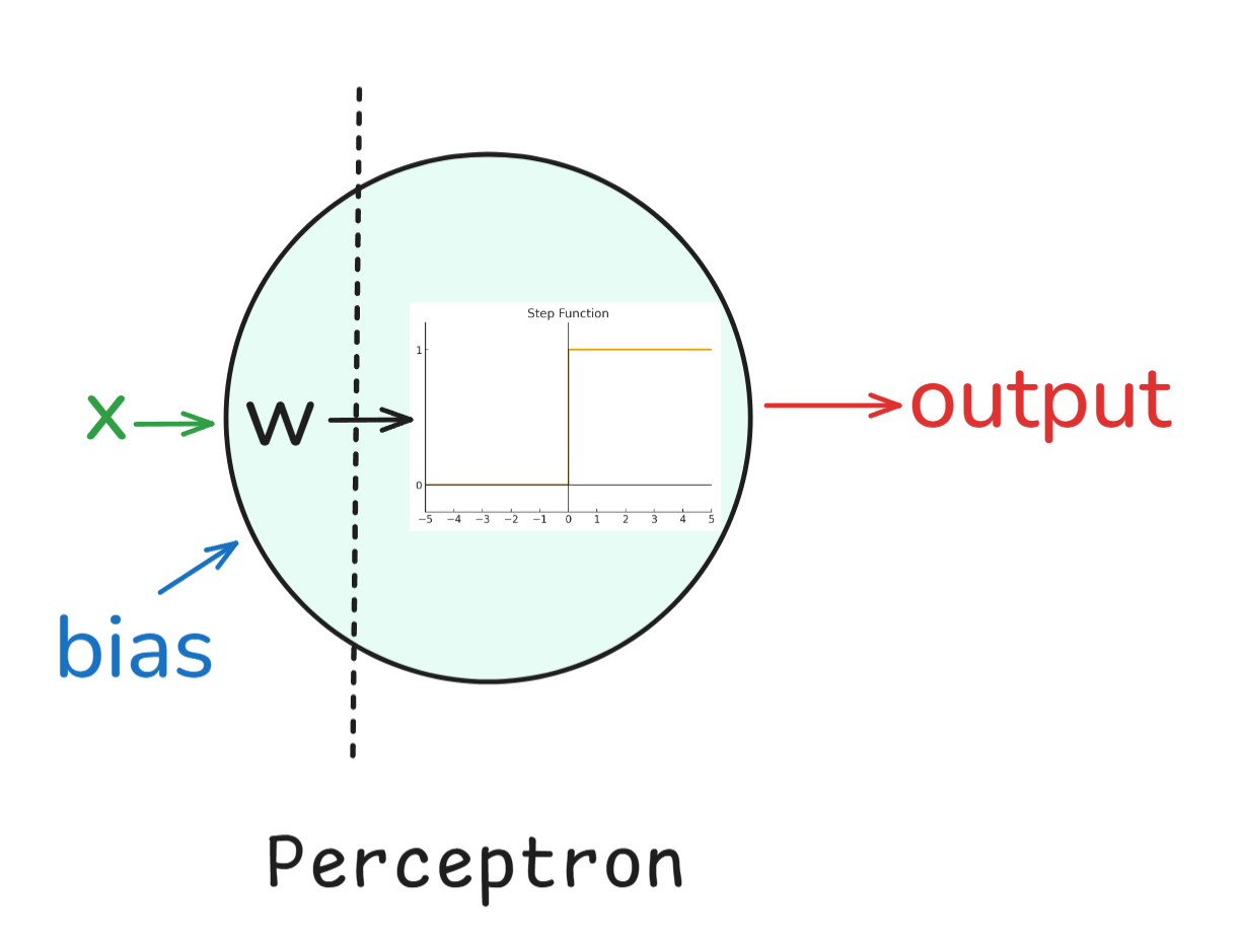
Essentially, the perceptron is a linear classifier, meaning that it could only draw straight-line (or hyperplane) decision boundaries. On the one hand, the Perceptron had its merits such as being very simple and elegant (since it was inspired by biology) as well as being computationally cheap. On the other hand though, it could not solve problems which are not linearly separable, such as the XOR problem. 

Multi-Layer Perceptrons (MLPs): Fast-forwarding a few decades, in the 1980s, researchers figured out that if you stacked multiple perceptrons and added non-linear activation functions, you could solve more complex problems. This structure became known as the Multi-Layer Perceptron.

Here is how it worked: 

1. Input Layer: Took in raw features from the dataset.
2. Hidden Layers: One or more layers of perceptrons that apply transformations. Each neuron performed z = w*x + b and passed it through a non-linear activation function such as sigmoid, tanh, etc. 
3. Output Layer: The final layer produced the final prediction (e.g., class probabilities, regression values).

The addition of these non-linear activations was crucial. Without them, stacking layers would just collapse into a single linear transformation. With them, MLPs could represent highly complex, non-linear functions.

This led to one of the most famous results in neural network theory: the Universal Approximation Theorem. 

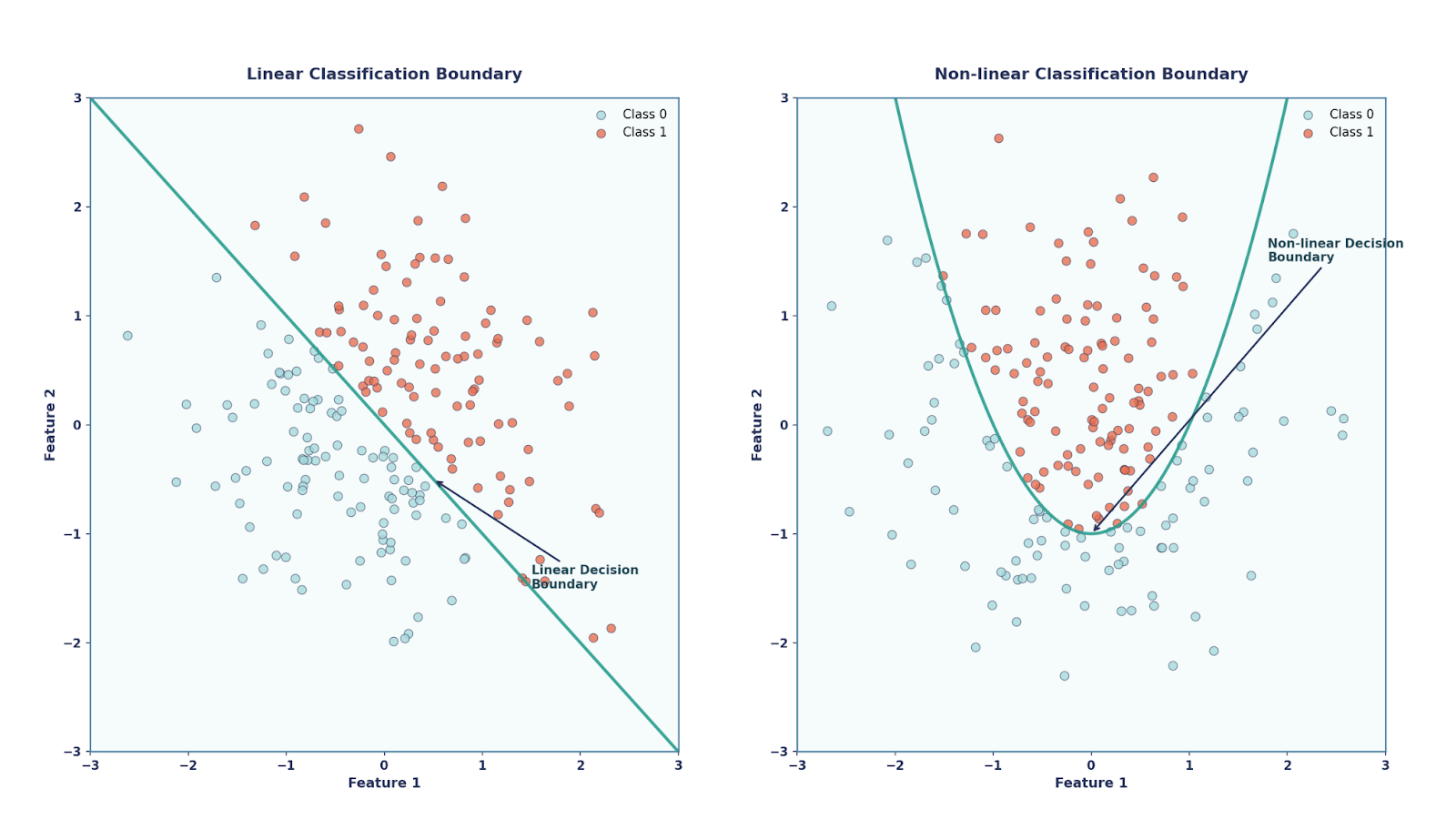
This theorem states that a neural network with even just a single hidden layer — as long as it has a non-linear activation function and enough neurons — can approximate any continuous function on a bounded domain. 

Deep Learning Era: Progressing to the 2010s, we enter the deep learning era. With GPUs and big data, FFNNs evolved into deeper and more powerful architectures, forming the foundation for CNNs, RNNs, and Transformers, which is where we are essentially at now.

So, going back to the original misconception now, we now know:

• Feed-Forward Neural Network (FFNN). The general category of any neural network where data flows in one direction (input → hidden → output), no loops.
• Multi-Layer Perceptron (MLP). A type of FFN that specifically has at least one hidden layer of perceptrons (neurons with weights, bias, and activation).

In other words, all MLPs are FFNNs, but not all FFNNs are MLPs. This is a very important point to remember. Another common misconception is about a single-layer perceptron (i.e., just input to output).

A single-layer perceptron is an FFNN, but not an MLP! Only once we add hidden layers, does it become an MLP.

This distinction is important as MLPs are capable of universal function approximation (with enough hidden units and non-linear activation functions), while simple single-layer perceptrons are limited in what they can represent.

Architecture of a Feed-Forward Neural Network

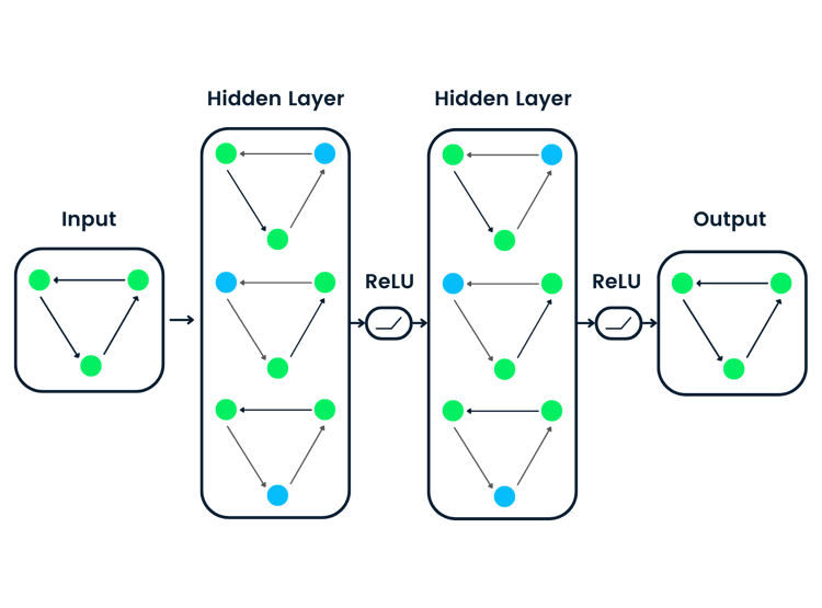
From the previous section, we learnt a lot about FFNN, but simply put they can be thought of as a stack of simple transformations. There are a lot of different components which create a FFNN so let’s explore these in more detail, in particular the MLP structure. 

In a MLP, there are three types of Layers; Input, Hidden and Output Layer, which we briefly mentioned before. 

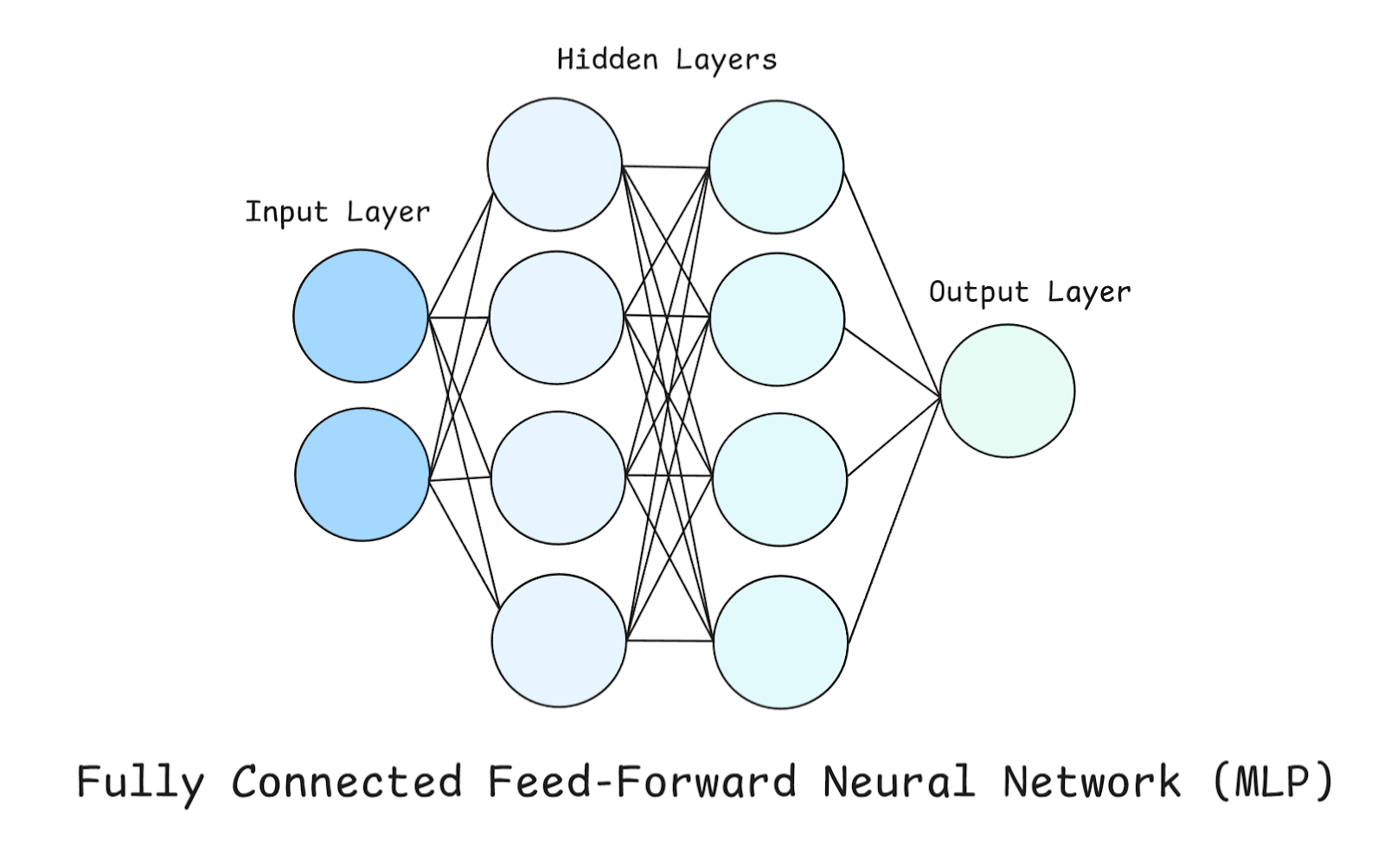
Take a look at the above diagram whilst we explore these layers in more detail. 

Input layer

This is the entry point of the network.  Each neuron here represents one feature from the dataset. Importantly, the input layer does not perform any computation itself — it simply passes raw numbers forward. In our example, since there are only two neurons in the Input Layer, this means that our dataset contains two features (or we are only considering two features from our dataset). 

Hidden layers

These are where the real computation happens. We have two Hidden layers, each containing four neurons. Each neuron in a hidden layer does these three things:

1. Weighted sum: Each input is multiplied by a weight and then all of them are summed. 
2. Bias: A constant bias is added to give flexibility in shifting the function.
3. Activation function: A non-linear squashing function like ReLU, tanh, or sigmoid is applied. This step is what allows the network to learn complex, non-linear patterns.

Output layer

The output layer produces the final prediction, and its design depends on the problem we are trying to solve:

• Regression problems, such as predicting house prices. In this case, the output layer will contain one neuron with no activation (linear). Why linear? Because we don’t want to squash values,  house prices could be any real number.
• Binary classification problems (yes/no decisions), such as predicting whether an email is spam or not. Here, the output layer would be one neuron with a sigmoid activation. Why sigmoid? This is because we want our network to output values between 0 and 1 (since we are predicting probabilities). 
• Multi-class classification problems (3 or more classes) - such as classifying an image as different animals. The output layer would have one neuron per class, with softmax activation. Why softmax? Because it turns raw scores into probabilities that add up to 1 (e.g., 70% cat, 20% dog, 10% horse).

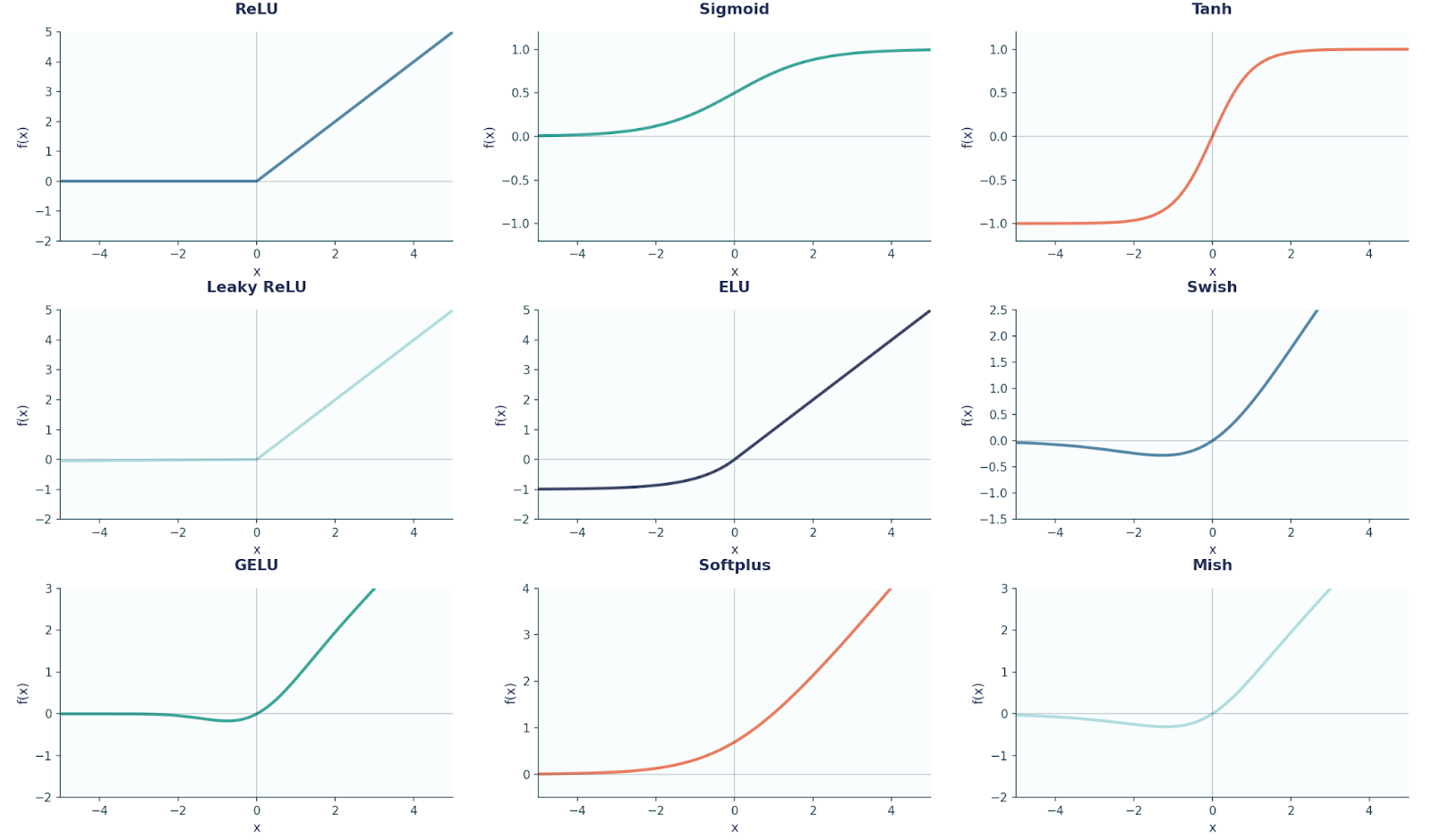
For your reference, here is a diagram showing nine common activation function shapes that are used in FFNN and Deep Learning in general. 

Before we move on, it is also important to note here that every neuron in one layer connects to every neuron in the next layer (that’s why it’s referenced as fully-connected). 

Going back to our example again, we have:

Params = (2⋅4+4)+(4⋅4+4)+(4⋅1+1)=12+20+5=37

Each bracket shows the number of parameters between consecutive layers, where the previous layer and current layer’s number of neurons are multiplied together and then the number of biases (i.e., number of neurons in current layer) are added as well. Try to perform these calculations on other neural network examples as well for practice!

Training a Feedforward Neural Network

In Deep Learning, training is split into two steps: forward pass/propagation and backpropagation. In simple words, Forward propagation gives us predictions, whereas Backpropagation is how we learn from mistakes. 

Forward propagation 

Everything we have covered so far is under forward propagation. To summarize, when data moves through an MLP, each layer performs the same two steps, which can be mathematically written by these equations:

Here z is the output after multiplying the previous layer’s output to the current layer’s weights and summing the bias, also known as the Linear Step. 

Naturally, if the previous layer is the input layer, then this would be x instead of al-1. The next step is the Activation Step. To make this more mathematically rigorous, we can write the Weights and Bias as these:

Backpropagation

When we have received an output, how do we tell our network if it is correct or not? Or better yet, how do we make the network better at our given task. This is where Backpropagation comes in. We can think of it as the feedback system for the network, where it tells the model how far off it was and how to adjust itself. We can break it down like this:

1. Compare predictions: Look at what the model predicted (ŷ) and what the true answer was (y).
2. Calculate the error: We use a loss function to measure how wrong the prediction was, such as MSE.
3. Backpropagate (via the chain rule): The gradients with respect to all of the bias and weights are computed. ∂L/∂w,∂L/∂b .
4. Gradient Descent update: The respective parameters are updated to reduce loss using the below rule:

Here, η is the learning rate, a parameter that can be changed to determine the amount the parameters should change by at every update. 

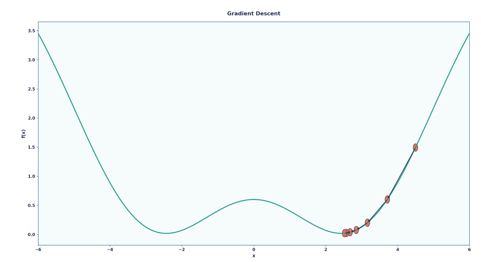
Over many rounds of this process, the network gradually learns and improves at the task.

To make things clearer, let’s walk through a very small example together. Suppose we have:

• Input: x = 2
• Target output: y=4
• Prediction: ŷ = 3

Now let’s go through the steps. 

1. Compare prediction: ŷ =3, y = 4
2. Error: For this example, we are going to be using the MSE: L=(y−y^​)2=(4−3)2=1
3. Backpropagate: The network figures out how much each weight and bias caused this error using derivatives and then we update each of the parameters using the gradient descent update step. 

Coding a Feed Forward Neural Network in PyTorch

We have covered the relevant mathematics to build a FFNN (specifically a MLP). To progress further, we are going to code this in PyTorch. 

Multilayer perceptron

# Imports we will be needing
import torch
import torch.nn as nn
import torch.optim as optim

X,y = dataset # Here will be our dataset 

# We have created a MLP here using nn.Sequential()
model = nn.Sequential(
    nn.Linear(2, 4),  # input layer → hidden layer (2 → 4)
    nn.ReLU(),        # relu activation function
    nn.Linear(4, 4), # hidden layer 1 → hidden layer 2 (4 → 4)
    nn.ReLU(), 
    nn.Linear(4, 1)   # hidden layer 2 → output (4 → 1)
)


criterion = nn.MSELoss()         # regression loss, i.e our loss function
optimizer = optim.SGD(model.parameters(), lr=0.1) # Optimizer using the Stochastic Gradient Descent

# Training Loop
EPOCHS = 200 # Number of epochs we will be training for
for epoch in range(EPOCHS):
    # Forward pass
    outputs = model(X)
    loss = criterion(outputs, y)

    # Backward pass
    optimizer.zero_grad()
    loss.backward()
    optimizer.step()

At this point, you should be able to map the PyTorch code to the mathematical steps we explored before. However, you could have a question regarding Epochs.

An epoch is one complete pass of the entire training dataset through the neural network. For example, let's suppose we had 1,000 training data points and batch size = 100, then after the network has seen all 1,000 images (i.e 10 batches), that’s 1 epoch. Training usually takes many epochs so the model can keep improving its weights.

Convolutional neural network

I also want to briefly mention other FFNNs as well, a very famous one being the Convolutional Neural Network (CNN). 

Although a CNN also contains an MLP at the end, at the start, it contains these special layers called Convolutional Layers and Pooling Layers. Talking about Convolutional Layers first, these are essential since they look only at small local regions of the input at a time using a filter (or kernel).

This is really useful when classifying images since:

• Dense layers would have treated every pixel as separate, ignoring spatial structure.
• Convolutional layers, on the other hand, can detect edges, textures, and shapes in small patches — then combine them into more complex patterns as we go deeper.

Alongside convolutional layers, CNNs also use pooling layers.

It is important to note that Pooling layers don’t learn parameters, but instead downsample the feature maps to make them smaller and more manageable.

• The most common is Max Pooling, which takes the maximum value from each small region (e.g., a 2×2 window).
• Pooling makes the network more efficient and also gives translation invariance (the network cares more about whether a feature exists, not exactly where it is).

We can code a CNN using PyTorch like such:

class SimpleCNN(nn.Module): # Define our model as a class
    def __init__(self):
        super().__init__()
        self.conv = nn.Conv2d(1, 8, 3)     # 1→8 channels, 3x3 kernel
        self.pool = nn.MaxPool2d(2, 2)
        self.fc   = nn.Linear(8*13*13, 10) # flatten → 10 classes

    def forward(self, x): # Forward propagation function 
        x = self.pool(torch.relu(self.conv(x)))
        x = x.view(x.size(0), -1)          # flatten
        return self.fc(x)

In the above code, we have created a very simple CNN, consisting of a single convolution layer, a single pooling layer, and a single linear layer. 

Other examples of feed-forward neural networks

We have covered two very famous and important examples of FFNNs, but there are many more such examples which have been revolutionary in their own respective domains, such as:

1. Transformers: each block contains an MLP/FFN part (after self-attention, the "feed-forward layer" expands + shrinks dimensions).
2. Vision Transformers (ViTs): apply transformer blocks (with FFNNs inside) to image patches.
3. Autoencoders (basic ones): encoder + decoder both built from FFNNs.
4. Recommender systems (MLP-based): e.g. Wide & Deep models for ranking and predictions.

Final Thoughts

Hopefully you have come to realise how important FFNNs are in the field of AI. Without these, the modern landscape of deep learning would not exist.

To continue I would highly recommend mastering backpropagation and going deeper into activation functions. Since this is the foundation to Deep Learning, I would also recommend learning Deep Learning with PyTorch.