TPOT in Python

In this tutorial, you will learn how to use a very unique library in python: tpot . The reason why this library is unique is that it automates the entire Machine Learning pipeline and provides you with the best performing machine learning model. More specifically, you will learn:

• The idea behind Automated Machine Learning
• How TPOT uses Genetic Programming to select the best machine learning model
• Using TPOT on a dataset in Python
• Limitations of TPOT

Let's get started!

Introduction

There are a lot of components you have to consider before solving a machine learning problem some of which includes data preparation, feature selection, feature engineering, model selection and validation, hyperparameter tuning, etc. In theory, you can find and apply a plethora of techniques for each of these components, but they all might perform differently for different datasets. The challenge is to find the best performing combination of techniques so that you can minimize the error in your predictions. This is the main reason that nowadays people are working to develop Auto-ML algorithms and platforms so that anyone, without any machine learning expertise, can build models without spending much time or effort. One such platform is available as a python library: TPOT. You can consider TPOT your Data Science Assistant. TPOT is a python Automated Machine Learning tool that optimizes machine learning pipelines using genetic programming. It will automate the most tedious part of machine learning by intelligently exploring thousands of possible pipelines to find the best one for your data.

from IPython.core.display import Image
Image(filename="/home/manishpathak/DataCamp/tpot/tpot-ml-pipeline.png",width=800,height=800)

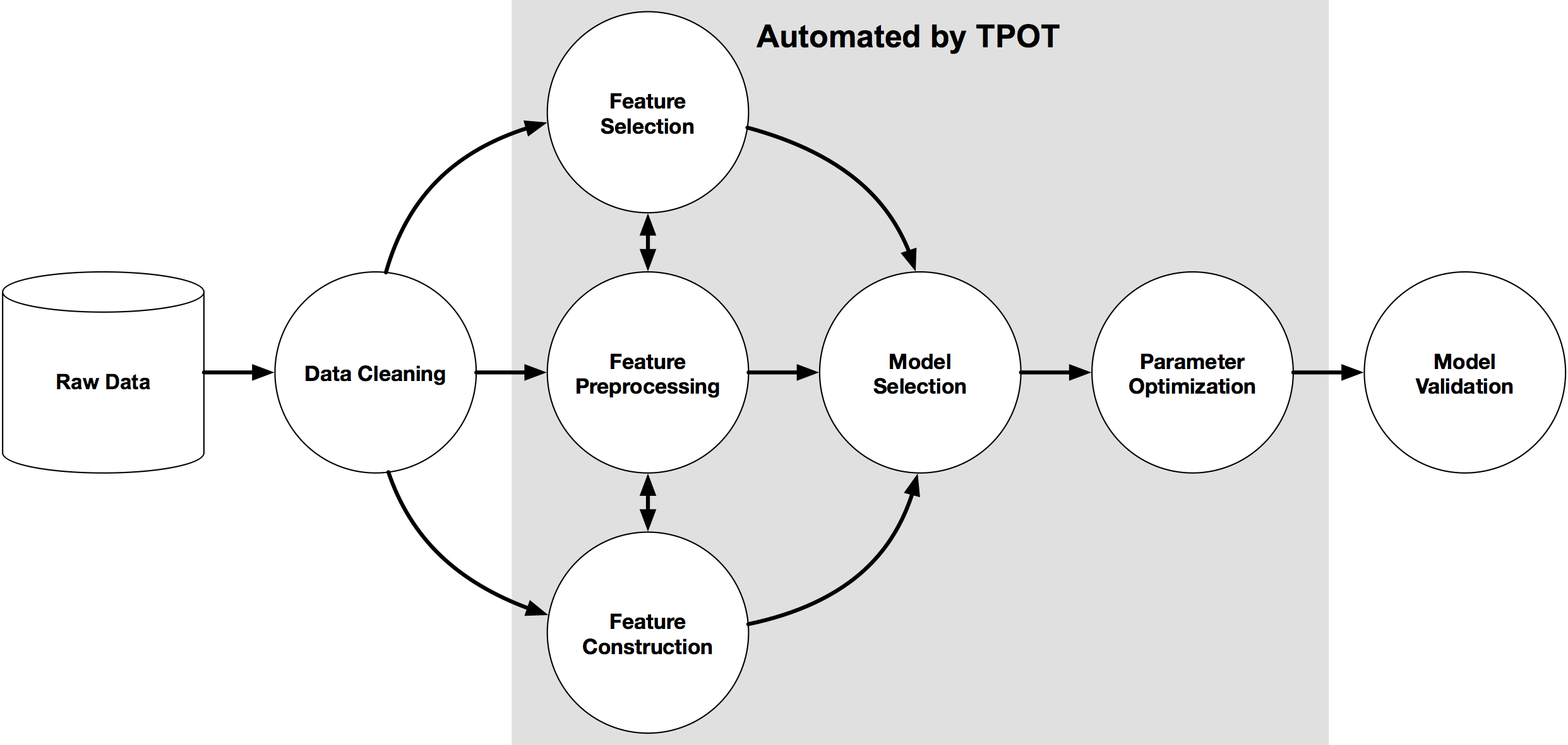
Once TPOT is finished searching, it provides you with the Python code for the best pipeline it found so you can tinker with the pipeline from there.

Installation

To install tpot on your system, you can run the command sudo pip install tpot on command line terminal or check out this link. tpot is built on top of several existing Python libraries, including numpy, scipy, scikit-learn, DEAP, update_checker, tqdm, stopit, pandas. Most of the necessary Python packages can be installed via the Anaconda Python distribution, or you could install them separately also. Optionally, you can also install XGBoost if you would like tpot to use the eXtreme Gradient Boosting models.

Genetic Programming

With the right data, computing power and machine learning model you can discover a solution to any problem, but knowing which model to use can be challenging for you as there are so many of them like Decision Trees, SVM, KNN, etc. That's where genetic programming can be of great use and provide help. Genetic algorithms are inspired by the Darwinian process of Natural Selection, and they are used to generate solutions to optimization and search problems in computer science.

Broadly speaking, Genetic Algorithms have three properties:

• Selection: You have a population of possible solutions to a given problem and a fitness function. At every iteration, you evaluate how to fit each solution with your fitness function.
• Crossover: Then you select the fittest ones and perform crossover to create a new population.
• Mutation: You take those children and mutate them with some random modification and repeat the process until you get the fittest or best solution.

Genetic Programming itself is a big topic in computer science but if you wish to go deeper into genetic algorithms, check out this video series.

But how does this all fit into data science?

Well, it turns out that choosing the right machine learning model and all the best hyperparameters for that model is itself an optimization problem for which genetic programming can be used. The Python library tpot built on top of scikit-learn uses genetic programming to optimize your machine learning pipeline. For instance, in machine learning, after preparing your data you need to know what features to input to your model and how you should construct those features. Once you have those features, you input them into your model to train on, and then you tune your hyperparameters to get the optimal results. Instead of doing this all by yourselves through trial and error, TPOT automates these steps for you with genetic programming and outputs the optimal code for you when it's done.

To understand further, you will practice using the tpot library on an open source dataset. The dataset you will be using is MAGIC Gamma Telescope DataSet. The data are generated to simulate registration of high energy gamma particles in a ground-based atmospheric Cherenkov gamma telescope using the imaging technique. To get full details about the dataset description check out this link. The dataset has the following attributes/features :

1. fLength: continuous # major axis of ellipse [mm]
2. fWidth: continuous # minor axis of ellipse [mm]
3. fSize: continuous # 10-log of sum of content of all pixels [in #phot]
4. fConc: continuous # ratio of sum of two highest pixels over fSize [ratio]
5. fConc1: continuous # ratio of highest pixel over fSize [ratio]
6. fAsym: continuous # distance from the highest pixel to center, projected onto major axis [mm]
7. fM3Long: continuous # 3rd root of the third moment along major axis [mm]
8. fM3Trans: continuous # 3rd root of the third moment along minor axis [mm]
9. fAlpha: continuous # angle of major axis with a vector to origin [deg]
10. fDist: continuous # distance from the origin to the center of the ellipse [mm]
11. class: g,h # gamma (signal), hadron (background) (target variable)

The goal is to classify an observation as gamma, which is the desired signal, or hadron, which is the background noise, based on the attributes provided.

You will start by importing pandas and numpy libraries to read the data and perform computations on it respectively.

import pandas as pd
import numpy as np

Use the pandas read_csv() function to read the dataset as a DataFrame. Also, specify the parameter header = None since the dataset doesn't have column names yet.

telescope_data=pd.read_csv('https://archive.ics.uci.edu/ml/machine-learning-databases/magic/magic04.data',header=None)

Check the contents of the DataFrame using the head() method.

telescope_data.head()

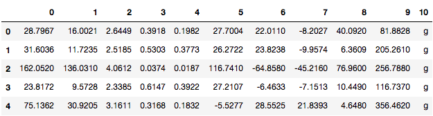
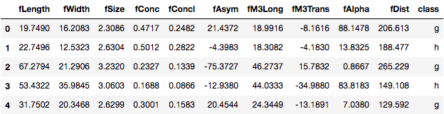
To give names to the columns of the DataFrame, you can use the attribute columns on the pandas DataFrame and assign it to a list containing the names of the columns.

telescope_data.columns = ['fLength', 'fWidth','fSize','fConc','fConcl','fAsym','fM3Long','fM3Trans','fAlpha','fDist','class']

telescope_data.head()

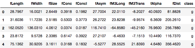
Now you have the column names as well in your DataFrame.

To get the necessary information about the DataFrame like the number of values in each column, data-type, count, mean, etc., you can use the pandas info() and describe() methods.

telescope_data.info()

<class 'pandas.core.frame.DataFrame'>
RangeIndex: 19020 entries, 0 to 19019
Data columns (total 11 columns):
fLength     19020 non-null float64
fWidth      19020 non-null float64
fSize       19020 non-null float64
fConc       19020 non-null float64
fConcl      19020 non-null float64
fAsym       19020 non-null float64
fM3Long     19020 non-null float64
fM3Trans    19020 non-null float64
fAlpha      19020 non-null float64
fDist       19020 non-null float64
class       19020 non-null object
dtypes: float64(10), object(1)
memory usage: 1.6+ MB

telescope_data.describe()

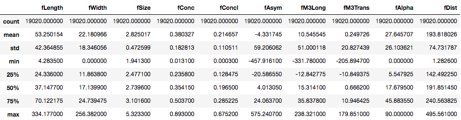
Turns out all the features in the DataFrame are continuous in nature. The target variable/feature class is however categorical. You can check the counts of each class in the target variable using value_counts() method.

telescope_data['class'].value_counts()

g    12332
h     6688
Name: class, dtype: int64

It's generally a good idea to randomly shuffle the data before starting to avoid any type of ordering in the data. You can rearrange the data in the DataFrame using numpy's random and permutation() function. To reset the index numbers after the shuffle use reset_index() method with drop = True as a parameter.

telescope_shuffle=telescope_data.iloc[np.random.permutation(len(telescope_data))]
tele=telescope_shuffle.reset_index(drop=True)
tele.head()

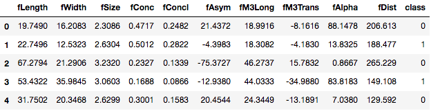
Before using tpot, it is essential you do the labeling of categorical variables in your DataFrame. To learn more about labeling categorical variables check out this tutorial. Here only the target variable class is the categorical feature, hence the treatment should be done to that column. You will replace the g class (signal) with a numerical value 0 and h class (background) with numerical value 1. This can be achieved via map() function with the argument as a dictionary which holds the respective mapping of the classes of the target variable.

tele['class']=tele['class'].map({'g':0,'h':1})

tele.head()

Now you store the class labels, which you need to predict, in a separate variable tele_class.

tele_class = tele['class'].values

You should also do missing value treatment before using tpot. To check the number of missing values column-wise, you can execute the following:

pd.isnull(tele).any()

fLength     False
fWidth      False
fSize       False
fConc       False
fConcl      False
fAsym       False
fM3Long     False
fM3Trans    False
fAlpha      False
fDist       False
class       False
dtype: bool

This dataset doesn't have any missing values. Note in datasets with missing values you can either drop the rows/columns using dropna() method or replace the missing value with some dummy value using fillna() method. For example, the following chunk of code will replace the NA values with a dummy value -999.

tele = tele.fillna(-999)

You will now split the DataFrame into a training set and a testing set just like you do while doing any type of machine learning modeling. You can do this via sklearn's cross_validation train_test_split. The parameters are tele.index as indexes of the DataFrame, train_size = 0.75 to keep 75% of the data in training set, test_size = 0.25 to keep the rest 25% data in testing set and stratify = tele_class the class label's values in the dataset. Note the validation set is just to give us an idea of the test set error. Here it is kept to be the same as a test set.

from sklearn.cross_validation import train_test_split
training_indices, validation_indices = training_indices, testing_indices = train_test_split(tele.index,
                                                                                            stratify = tele_class,
                                                                                            train_size=0.75, test_size=0.25)

You can check the size of the training set and validation set using the size attribute.

training_indices.size, validation_indices.size

(14265, 4755)

Now it's time to use the tpot library to suggest us the best pipeline for this binary classification problem. To do so, you have to import TPOTClassifier class from the tpot library. Had this been a regression problem you would have imported TPOTRegressor class.

TPOTClassifier has a wide variety of parameters, and you can read all about them here. But the most notable ones you must know are:

• generations: Number of iterations to the run pipeline optimization process. The default is 100.
• population_size: Number of individuals to retain in the genetic programming population every generation. The default is 100.
• offspring_size: Number of offspring to produce in each genetic programming generation. The default is 100.
• mutation_rate: Mutation rate for the genetic programming algorithm in the range [0.0, 1.0]. This parameter tells the GP algorithm how many pipelines to apply random changes to every generation. Default is 0.9
• crossover_rate: Crossover rate for the genetic programming algorithm in the range [0.0, 1.0]. This parameter tells the genetic programming algorithm how many pipelines to "breed" every generation.
• scoring: Function used to evaluate the quality of a given pipeline for the classification problem like accuracy, average_precision, roc_auc, recall, etc. The default is accuracy.
• cv: Cross-validation strategy used when evaluating pipelines. The default is 5.
• random_state: The seed of the pseudo-random number generator used in TPOT. Use this parameter to make sure that TPOT will give you the same results each time you run it against the same data set with that seed.

Also note mutation_rate + crossover_rate cannot exceed 1.0.

Here you will use tpot with generations = 5 and the rest of the parameters at default values. The parameter verbosity = 2 states how much information TPOT communicates while it's running.

Then you will call the fit() method with the training set (without the target column) and the target column as the arguments.

Note running the code in the below cell will take several hours to finish. With the given TPOT settings (5 generations with 100 population size), TPOT will evaluate 500 pipeline configurations before finishing. To put this number into context, think about a grid search of 500 hyperparameter combinations for a machine learning algorithm and how long that grid search will take. That is 500 model configurations to evaluate with 5-fold cross-validation, which means that roughly 2500 models are fit and evaluated on the training data in one grid search. That's a time-consuming procedure! Later, you will get to know about some more arguments that you can pass to TPOTClassifier to control the execution time for TPOT to finish.

from tpot import TPOTClassifier
from tpot import TPOTRegressor

tpot = TPOTClassifier(generations=5,verbosity=2)

tpot.fit(tele.drop('class',axis=1).loc[training_indices].values,
         tele.loc[training_indices,'class'].values)

Optimization Progress:  33%|███▎      | 200/600 [41:43<1:51:41, 16.75s/pipeline]

Generation 1 - Current best internal CV score: 0.880266061124

Optimization Progress:  50%|█████     | 300/600 [1:14:37<46:57,  9.39s/pipeline]  

Generation 2 - Current best internal CV score: 0.880266061124

Optimization Progress:  67%|██████▋   | 400/600 [1:59:17<2:21:21, 42.41s/pipeline]

Generation 3 - Current best internal CV score: 0.880266061124

Optimization Progress:  84%|████████▎ | 501/600 [3:01:12<1:02:16, 37.74s/pipeline]

Generation 4 - Current best internal CV score: 0.881597992166

Generation 5 - Current best internal CV score: 0.881597992166

Best pipeline: GradientBoostingClassifier(RobustScaler(PolynomialFeatures(input_matrix, degree=2, include_bias=False, interaction_only=False)), learning_rate=0.1, max_depth=6, max_features=0.6000000000000001, min_samples_leaf=12, min_samples_split=3, n_estimators=100, subsample=0.55)

TPOTClassifier(config_dict={'sklearn.ensemble.GradientBoostingClassifier': {'max_features': array([0.05, 0.1 , 0.15, 0.2 , 0.25, 0.3 , 0.35, 0.4 , 0.45, 0.5 , 0.55,
       0.6 , 0.65, 0.7 , 0.75, 0.8 , 0.85, 0.9 , 0.95, 1.  ]), 'learning_rate': [0.001, 0.01, 0.1, 0.5, 1.0], 'min_samples_leaf': [1, 2, 3, 4, 5, 6, 7...  0.6 , 0.65, 0.7 , 0.75, 0.8 , 0.85, 0.9 , 0.95, 1.  ])}, 'sklearn.preprocessing.RobustScaler': {}},
        crossover_rate=0.1, cv=5, disable_update_check=False,
        early_stop=None, generations=5, max_eval_time_mins=5,
        max_time_mins=None, memory=None, mutation_rate=0.9, n_jobs=1,
        offspring_size=100, periodic_checkpoint_folder=None,
        population_size=100, random_state=None, scoring=None,
        subsample=1.0, verbosity=2, warm_start=False)

In the above, 5 generations were computed, each giving the training efficiency of the fitting model on the training set. As evident, the best pipeline is the one that has the CV accuracy score of 88.16%. The model that produces this result is the pipeline, consisting of pre-processing techniques like PloynomialFeatures and then RobustScaler that adds synthetic features to the input data and normalizes them, which then get utilized by a Gradient Boosting classifier to form the final predictions. You can also notice that tpot gives various hyper-parameter values like learning_rate,max_depth, etc., also along with the classifier.

Next, the test error is computed for validation purposes.

tpot.score(tele.drop('class',axis=1).loc[validation_indices].values,
           tele.loc[validation_indices, 'class'].values)

0.885173501577287

As can be seen, the test accuracy is 88.51%.

Finally, you can tell TPOT to export the corresponding Python code for the optimized pipeline to a text file with the export function:

tpot.export('tpot_MAGIC_Gamma_Telescope_pipeline.py')

True

## This is the pipeline that tpot generated: tpot_MAGIC_Gamma_Telescope_pipeline.py
import numpy as np
import pandas as pd
from sklearn.ensemble import GradientBoostingClassifier
from sklearn.model_selection import train_test_split
from sklearn.pipeline import make_pipeline
from sklearn.preprocessing import PolynomialFeatures, RobustScaler

# NOTE: Make sure that the class is labeled 'target' in the data file
tpot_data = pd.read_csv('PATH/TO/DATA/FILE', sep='COLUMN_SEPARATOR', dtype=np.float64)
features = tpot_data.drop('target', axis=1).values
training_features, testing_features, training_target, testing_target = \
            train_test_split(features, tpot_data['target'].values, random_state=42)

# Score on the training set was:0.881597992166
exported_pipeline = make_pipeline(
    PolynomialFeatures(degree=2, include_bias=False, interaction_only=False),
    RobustScaler(),
    GradientBoostingClassifier(learning_rate=0.1, max_depth=6, max_features=0.6, min_samples_leaf=12, min_samples_split=3, n_estimators=100, subsample=0.55)
)

exported_pipeline.fit(training_features, training_target)
results = exported_pipeline.predict(testing_features)

Isn't that awesome? Without you tweaking a lot of parameters and options to get the best model, TPOT not only gave you the information about the best model but also a working code for it!

As indicated earlier, the last TPOT run took several hours to finish. Well, there are certain parameters you can specify to control the execution time of TPOT but with a trade-off. Since you will be limiting the time of TPOT execution, TPOT won't be able to explore all the possible pipelines and hence the best model suggested by TPOT at the end of the constrained time limit may not be the best model possible for that dataset. However, if sufficient time is given it will be somewhat closer to the best possible model. Some parameters are:

• max_time_mins: how many minutes TPOT has to optimize the pipeline. If not None, this setting will override the generations parameter and allow TPOT to run until max_time_mins minutes elapse.
• max_eval_time_mins: how many minutes TPOT has to evaluate a single pipeline. Setting this parameter to higher values will enable TPOT to evaluate more complex pipelines, but will also allow TPOT to run longer. Use this parameter to help prevent TPOT from wasting time on assessing time-consuming pipelines. The default is 5.
• early_stop: how many generations TPOT checks whether there is no improvement in the optimization process. Ends the optimization process if there is no improvement in the given number of generations.
• n_jobs: Number of procedures to use in parallel for evaluating pipelines during the TPOT optimization process. Setting n_jobs=-1 will use as many cores as available on the computer. Beware that using multiple methods on the same machine may cause memory issues for large datasets. The default is 1.
• subsample: Fraction of training samples that are used during the TPOT optimization process. Must be in the range (0.0, 1.0]. The default is 1.

Just for practice, you will again run TPOT with additional arguments max_time_mins = 2 and max_eval_time_mins = 0.04 but this time with reduced population_size = 15.

tpot = TPOTClassifier(verbosity=2, max_time_mins=2, max_eval_time_mins=0.04, population_size=15)
tpot.fit(tele.drop('class',axis=1).loc[training_indices].values, tele.loc[training_indices,'class'].values)

Optimization Progress: 42pipeline [00:42,  1.17s/pipeline]                  

Generation 1 - Current best internal CV score: 0.86119902629

Optimization Progress: 64pipeline [01:03,  1.04s/pipeline]                  

Generation 2 - Current best internal CV score: 0.86119902629

Optimization Progress: 83pipeline [01:21,  1.14s/pipeline]

Generation 3 - Current best internal CV score: 0.861689811492

Optimization Progress: 104pipeline [01:45,  1.03pipeline/s]

Generation 4 - Current best internal CV score: 0.861759642796

2.03228221667 minutes have elapsed. TPOT will close down.
TPOT closed prematurely. Will use the current best pipeline.

Best pipeline: XGBClassifier(RobustScaler(SelectPercentile(input_matrix, percentile=85)), learning_rate=0.1, max_depth=2, min_child_weight=4, n_estimators=100, nthread=1, subsample=0.1)

TPOTClassifier(config_dict={'sklearn.ensemble.GradientBoostingClassifier': {'max_features': array([0.05, 0.1 , 0.15, 0.2 , 0.25, 0.3 , 0.35, 0.4 , 0.45, 0.5 , 0.55,
       0.6 , 0.65, 0.7 , 0.75, 0.8 , 0.85, 0.9 , 0.95, 1.  ]), 'learning_rate': [0.001, 0.01, 0.1, 0.5, 1.0], 'min_samples_leaf': [1, 2, 3, 4, 5, 6, 7...  0.6 , 0.65, 0.7 , 0.75, 0.8 , 0.85, 0.9 , 0.95, 1.  ])}, 'sklearn.preprocessing.RobustScaler': {}},
        crossover_rate=0.1, cv=5, disable_update_check=False,
        early_stop=None, generations=1000000, max_eval_time_mins=0.04,
        max_time_mins=2, memory=None, mutation_rate=0.9, n_jobs=1,
        offspring_size=15, periodic_checkpoint_folder=None,
        population_size=15, random_state=None, scoring=None, subsample=1.0,
        verbosity=2, warm_start=False)

As you can notice the best performing classifier within the time frame specified is now XGBoost with SelectPercentile() and RobustScaler() as the pre-processing steps.

Limitations

• TPOT can take a long time to finish its search

Running TPOT isn’t as simple as fitting one model on the dataset. It is considering multiple machine learning algorithms (random forests, linear models, SVMs, etc.) in a pipeline with numerous preprocessing steps (missing value imputation, scaling, PCA, feature selection, etc.), the hyper-parameters for all of the models and preprocessing steps, as well as multiple ways to ensemble or stack the algorithms within the pipeline. That’s why it usually takes a long time to execute and isn’t feasible for large datasets.

• TPOT can recommend different solutions for the same dataset

If you're working with a reasonably complex dataset or run TPOT for a short amount of time, different TPOT runs may result in different pipeline recommendations. When two TPOT runs recommend different pipelines, this means that the TPOT runs didn't converge due to lack of time or that multiple pipelines perform more-or-less the same on your dataset.

Conclusion

Hurray! You have come to the end of this tutorial. You started with a little introduction about the idea behind Automated Machine Learning platforms. Then you explored a bit on Genetic Programming and how TPOT uses it to automate the machine learning pipeline building process. You also practiced using the TPOT library in Python on a dataset along with gaining knowledge about the functions it provides. If you plan to use TPOT in the future, I strongly suggest you look at its excellent documentation. Happy Exploring!

If you would like to learn more about Machine Learning in Python, take DataCamp's Machine Learning with Tree-Based Models in Python course. Also, check out DataCamp's Introduction to Machine Learning in Python tutorial.
 

The following web pages were used as sources in writing this tutorial.

• Classification
• What to expect from AutoML software