Coefficient of Determination: What R-Squared Tells Us

Imagine you’re trying to predict someone’s exam score based on how many hours they studied. Now, how well does your prediction match the actual scores? That’s what the coefficient of determination, also known as R^² (R-squared), tells us.

It tells us how much of the change in one thing (such as exam scores) can be explained by changes in another (such as study hours). This way, you can understand how well your model "fits" the data.

In this article, we’ll help you understand what R^² means, why it matters, and how to calculate and interpret it even if you're new to statistics. 

What Is the Coefficient of Determination?

The coefficient of determination, usually written as R^² (R-squared), is a number that tells us how well a regression model explains what’s going on in the data. It shows how much of the change in the outcome (dependent variable) can be explained by the things we’re using to predict it (independent variable(s)). 

Suppose you want to predict someone’s weight based on their height. If R^² is close to 1, your prediction is doing a great job. Most of the differences in weight can be attributed to differences in height. If R^² is close to 0, then your prediction is basically guessing because, in that case, height doesn’t explain much of the change in weight.

We expect R^² values between 0 and 1:

• 0 means the model explains none of the variability in the data.

• 1 means the model explains all of the variability.

• Values closer to 1 mean a better fit, which shows your model is capturing more of the pattern in the data.

Simple linear regression

When you're working with only one independent variable, the model is called a simple linear regression. In this case, R^² has a neat relationship with the Pearson correlation coefficient (r): R^² = r^²

This means if there’s a strong positive or negative correlation between your predictor and the outcome, R^² will be high.

Note: In models with more than one predictor (called multiple regression), R^² still tells you how much variance is explained, but it’s not just r^² anymore, because now you're combining the effects of multiple variables.

Can the coefficient of determination be negative?

R^² usually ranges from 0 to 1. But sometimes, you may see a negative R^². This can happen if:

• Your model doesn’t include an intercept (a constant starting value)
• You’re using the wrong type of model for the data

A negative R^² means your model is doing worse than guessing the average. In other words, it fits the data so poorly that it's actually misleading.

How to Calculate the Coefficient of Determination

There are two common ways to calculate R^²:

1. Using the sum of squares
2. Using the correlation coefficient (r)

Let’s walk through both.

Using the sum of squares

The most common formula for R^² is:

Here, the residual sum of squares (the unexplained part)) measures how far the actual values are from the predicted values made by your model. It’s the error your model makes.

The total sum of squares is the total variation in the observed data. It tells us how far the actual values are from the average (mean) of the dependent variable.

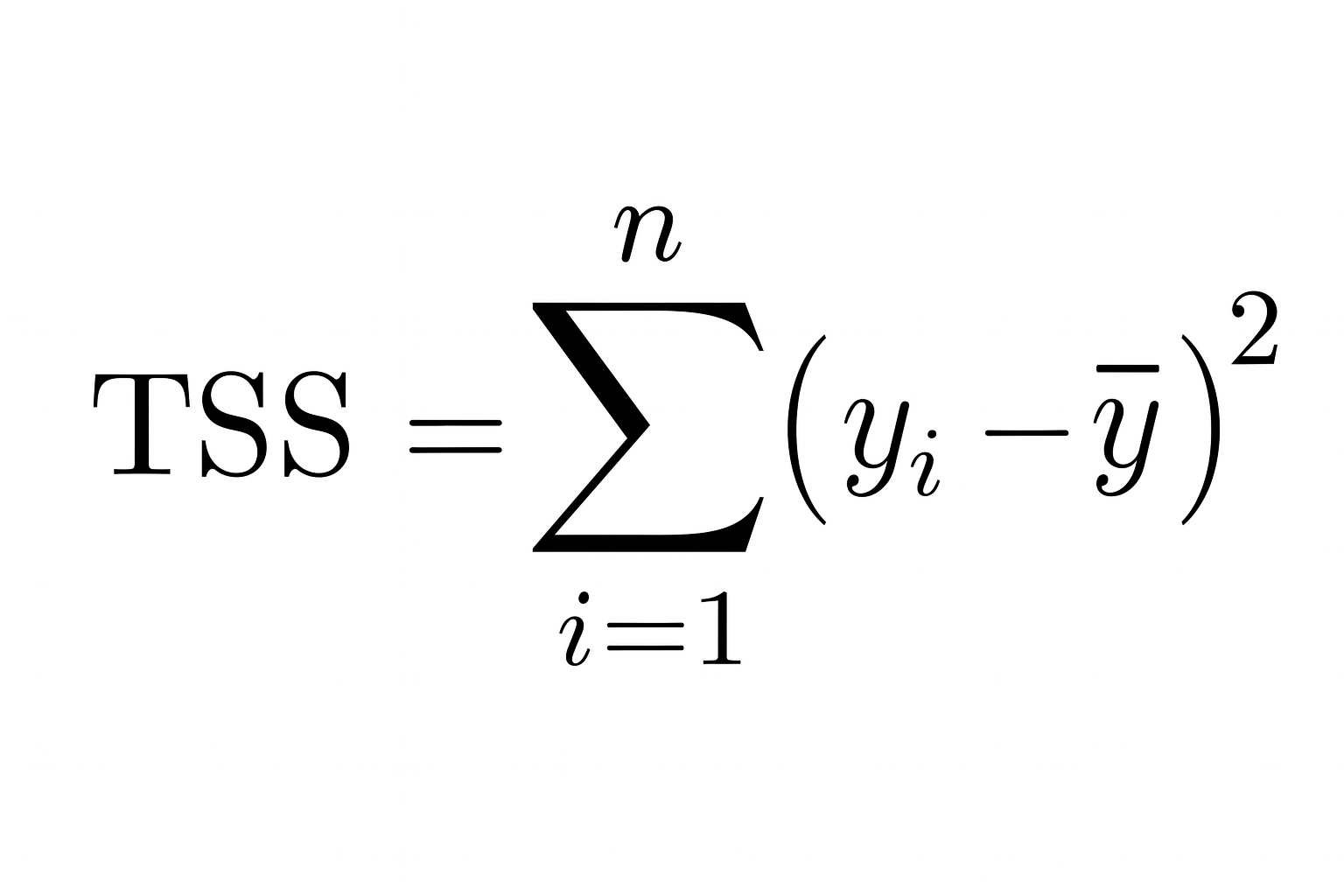
So, the smaller residual sum of squares is compared to the sum of squares total, the better your model fits the data, and the closer R^² gets to 1.

Let’s understand this with an example: 

Suppose you have a small dataset with the following values:

First, calculate the mean of actual values:

• y = (10+12+14)/3 = 12

Then calculate the sum of squares total (how far actual values are from the mean):

• sum of squares total = (10 − 12)² + (12 − 12)² + (14 − 12)² = 4 + 0 + 4 = 8

Next, calculate the residual sum of squares (how far actual values are from predicted values):

• residual sum of squares = (10 − 12)² + (12 − 11)² + (14 − 13)² = 4 + 1 + 1 = 6

Now add this to the formula:

• R^² = 1 − (residual sum of squares / total sum of squares) = 1 − (6/8) = 1 − 0.75 = 0.25

So, R^² = 0.25, which means the model explains 25% of the variation in the data.

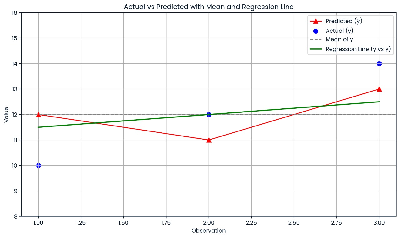
This chart shows how far each actual value is from its predicted value. The model’s predictions are off by a fair amount, which is why R² is just 0.25; only 25% of the variation is explained.

Using the correlation coefficient

If you’re using simple linear regression (only one independent variable), use this formula:

Here r is the Pearson correlation coefficient between the actual and predicted values. This shortcut only works when there’s a single predictor.

Let’s say the correlation between X and Y is: r = −0.8

Even though the correlation is negative (meaning the variables move in opposite directions), R^² is positive: R^² = (−0.8)^² = 0.64

So, 64% of the variation in the outcome can still be explained by the predictor, even if the relationship is negative. That’s why R^² is always positive or zero; it represents the amount of variation explained, not the direction.

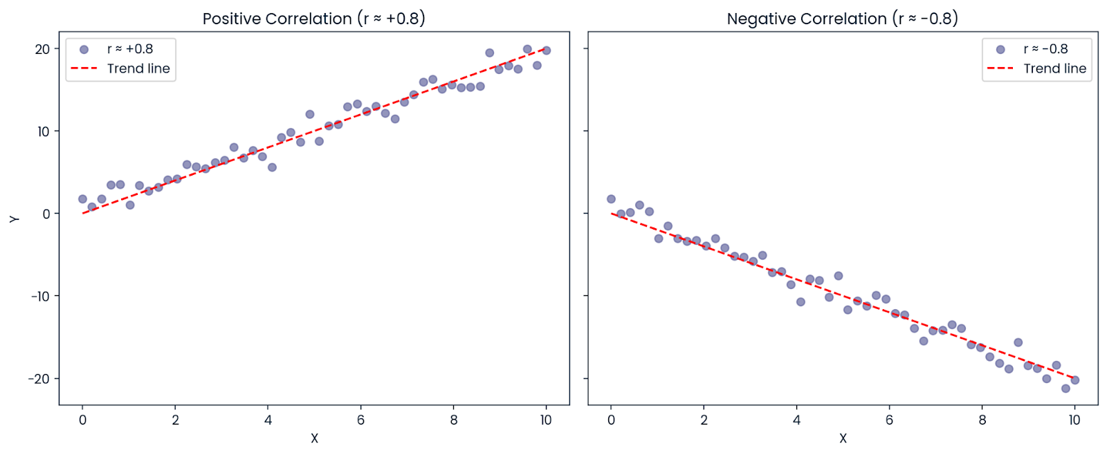
Positive and negative correlation. Image by Author.

How to Interpret the Coefficient of Determination

The coefficient of determination tells us how much of the variation in the outcome (dependent variable) is explained by our model. In simple terms, it's like asking: "How much of the changes in what I'm trying to predict can be explained by the data I'm using?"

Let’s say you're building a model to predict students’ exam scores based on how many hours they study. If your model gives you: R^² = 0.90

This means that 90% of the differences in exam scores can be explained by differences in study time. The other 10% comes from other factors your model didn’t include, like sleep, natural ability, prior knowledge, or test difficulty.

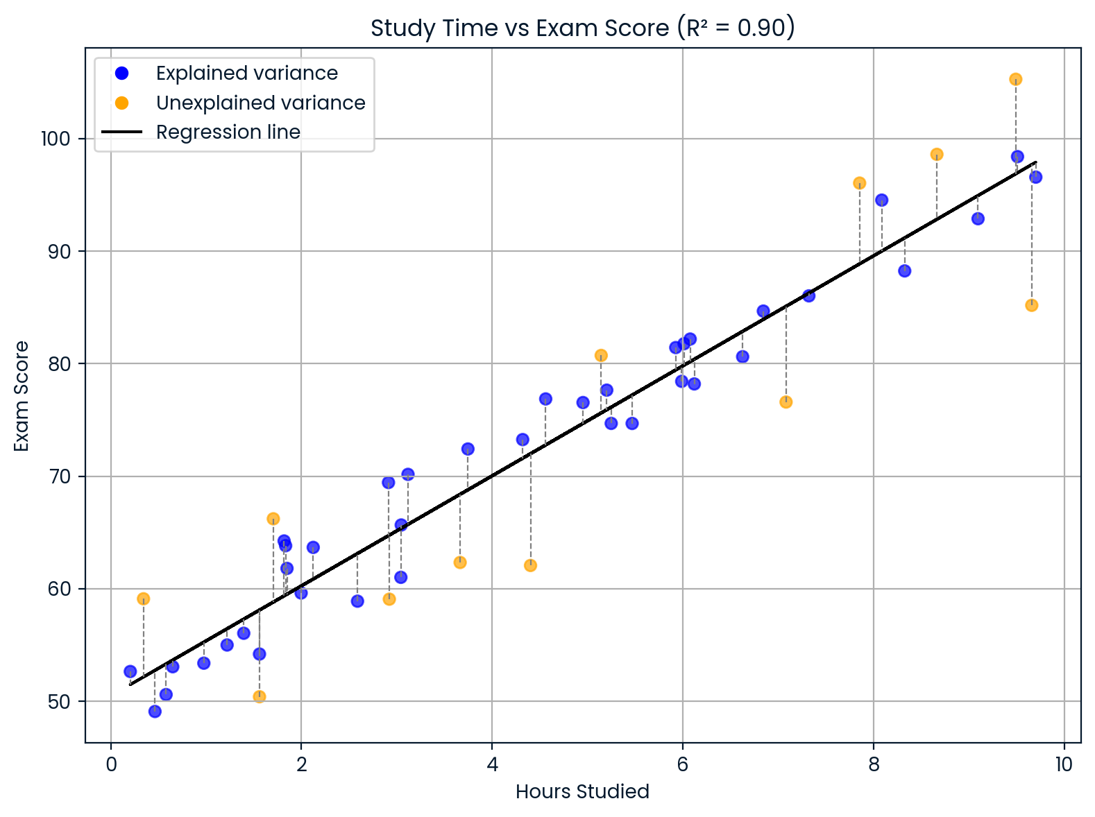
Interpreting the coefficient of determination. Image by Author.

This chart shows how study time affects exam scores. 

• The black line is the model’s prediction. 
• Blue dots are scores the model explained well using study time. 
• Orange dots represent scores that don’t fit, likely due to other factors such as sleep, test difficulty, or the student's prior knowledge. Since R^² = 0.90, most scores follow the pattern, but not all.

Cohen's guidelines

Jacob Cohen created a widely used guide to help us understand what different R^² values might mean when interpreting how strong a relationship is.

Here are Cohen’s rough benchmarks for R^²:

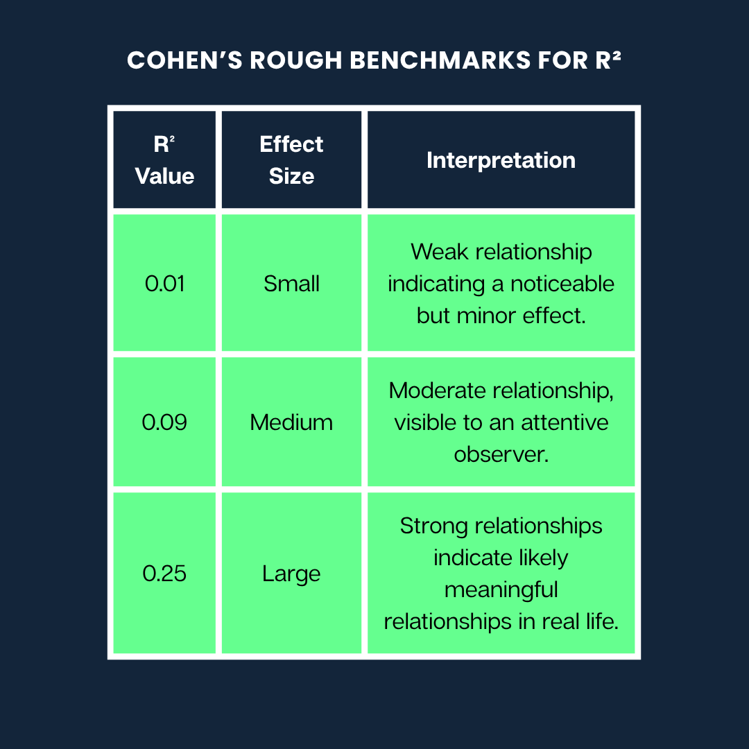
Cohen’s rough benchmarks. Image by Author

Note: These are general guidelines. What counts as a “large” or “small” effect can vary a lot depending on your field (like psychology vs. engineering) and the context of the research.

Limitations and Common Misconceptions

While R^² is helpful, you must understand what it can and can’t tell you. Here are some common misunderstandings and limitations to watch out for:

Myth 1: A high coefficient of determination means a better model

It may seem like a higher R^² always means a better model, but that’s not necessarily true. R^² always increases or stays the same when you add more variables to a model, even if those variables are completely irrelevant. 

Why? 

Because the model has more flexibility to fit the training data, even if it’s just fitting random noise. This can lead to overfitting, where your model looks great on the data it was trained on but performs poorly on new data.

Tip: Use adjusted R² when comparing models with different numbers of predictors. It penalizes unnecessary complexity and can help detect overfitting. 

Myth 2: A high coefficient of determination means accurate predictions on new data or causation

R^² only measures how well the model describes the data you already have. It does not tell you:

• If the model will make good predictions on new data
• Whether one variable causes the other

A high R^² can even happen by chance if you're using many predictors. So always look at other model evaluation metrics (like RMSE or MAE for prediction quality) and remember: correlation is not causation.

Myth 3: Low R-squared means the model is useless

Sometimes, in complex systems (like predicting human behavior or financial markets), a low R^² is expected.

For example, if you're modeling something influenced by many unpredictable or unmeasurable factors, your model may still be useful, even with a low R^². It might capture a meaningful trend or provide insights, even if it doesn’t explain a large portion of the variance.

In medical or psychological research, it’s common to see low R^² values because people’s outcomes depend on so many interacting variables.

Other Variants: Partial R-squared and Generalizations

While R^² helps understand how the model fits in linear regression, there are other variants and generalizations that help with different modeling contexts.

Adjusted R-squared

Like the regular R^², adjusted R^² tells us how much of the variation in the dependent variable is explained by the model. But it goes a step further by penalizing unnecessary complexity. In other words, it discourages you from stuffing your model with extra predictors that don’t help.

Its formula is:

Adjusted R² = 1 - [ (1 - R²) × (n - 1) / (n - p - 1) ]

Here:

• n is the number of observations (data points)

• p is the number of predictors (independent variables)

The formula adjusts R^² downward if a new variable doesn’t improve the model. This penalty becomes stronger as you add more predictors.

For example, if you add a new variable that improves your model’s accuracy, adjusted R^² will go up. But if that variable barely changes anything or only helps by chance, adjusted R^² will go down, alerting you to possible overfitting.

This makes adjusted R^² helpful for comparing models.

Let’s say you want to choose between a simpler model with three predictors and a more complex one with six. Even if the complex model has a slightly higher R^², the adjusted R^² might be lower, signaling that it’s not worth the added complexity.

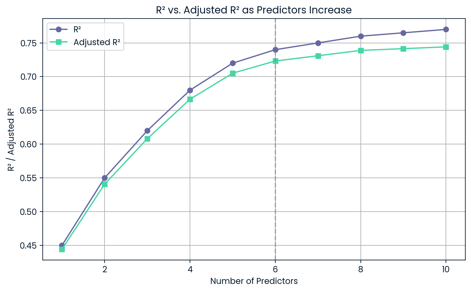
R² versus adjusted R² as predictors increase. Image by Author.

This chart shows that as you add more predictors, R^² keeps going up even if those predictors aren’t very useful. On the other hand, adjusted R^² drops if you add too much, warning you about overfitting.

Coefficient of partial determination

Partial R^² (or coefficient of partial determination) tells us how much additional variance in the dependent variable is explained by adding one specific predictor to a model that already includes others.

To calculate partial R^², we compare two models:

• The reduced model, which excludes the predictor in question
• The full model, which includes all predictors

The formula for partial R^² is based on the reduction in the Sum of Squared Errors (SSE) when the new variable is added. A common form is:

Or in terms of regression sums of squares:

Suppose you're building a model to predict product sales. 

You already have “product price” and “season” in the model. Now, you want to see if adding “marketing spend” improves predictions. Partial R² tells you how much more variance in sales is explained by including “marketing spend.”

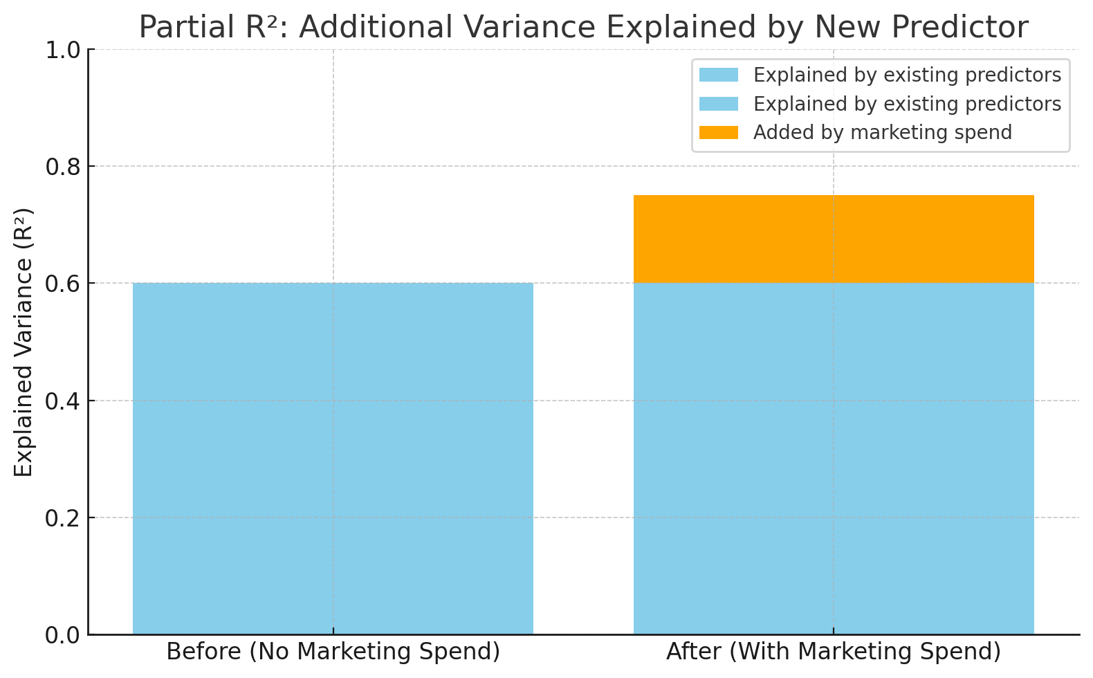
R^² increasing from 0.60 to 0.75 after adding marketing spend. Image by Author.

This chart shows how much more accurate the model becomes when “marketing spend” is added. R^² goes from 0.60 to 0.75, meaning the new variable explains 15% more of the variation in sales—that's the partial R^².

Coefficient of determination in logistic regression

In logistic regression, the outcome variable is categorical like yes/no, pass/fail so traditional R^² doesn't apply. Instead, we use pseudo-R^² metrics, which serve a similar purpose: to estimate how well the model explains the variation in outcomes.

Two common pseudo-R^² values are:

• Cox & Snell R^²: Estimates explained variance, but its maximum value is less than 1, even for a perfect model.
• Nagelkerke R^²: A corrected version of Cox & Snell R^² that scales up to 1, making it easier to interpret like traditional R^².

Suppose you're modeling whether a customer will click on an ad (yes/no). Because the outcome is binary, you can’t use regular R^². But pseudo-R^² values like Nagelkerke help compare logistic models and assess their predictive power, even if they aren’t directly equivalent to R^² in linear regression.

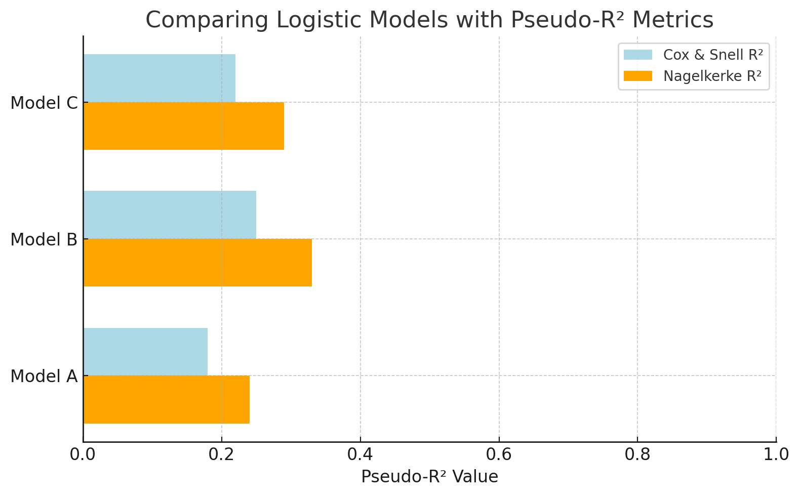
Compare logistics models with pseudo-R^² metrics. Image by Author.

This chart compares logistic regression models using pseudo-R^² values. Nagelkerke R^² offers a more interpretable scale than Cox & Snell. This makes it easier to evaluate how well each model explains the outcome (e.g., predicting ad clicks).

Coefficient of determination vs. other model fit metrics

While R^² is helpful for understanding how much variation is explained, it doesn’t measure how far off your predictions are. That’s what error-based metrics like RMSE, MAE, and MAPE help with.

Here’s a brief comparison:

Practical Applications Across Fields

Now, let’s look at a few of the countless cases where the coefficient of determination has been used. 

Economics: Explaining GDP fluctuations

In economics, R^² is used to explain changes in broad indicators like Gross Domestic Product (GDP). For example, a model may include variables like interest rates, consumer spending, and trade balances to predict GDP.

If such a model returns an R^² of 0.83, it means that 83% of the variation in GDP can be explained by these economic factors. This helps economists understand how much of the ups and downs in GDP can be attributed to known drivers.

A research study used U.S. GDP as an independent variable to predict the S&P 500 index and found an R^² of 0.83. This showed a strong relationship between economic activity and stock market trends.

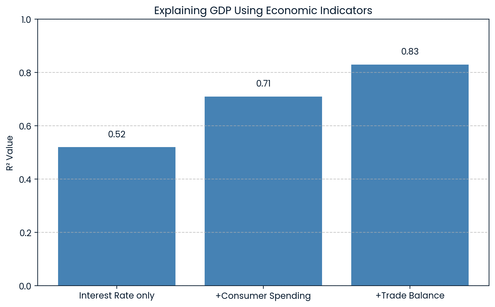
R^² explaining GDP economics. Image by Author.

The chart shows that as more economic indicators are added to the model, the R^² increases, from 0.52 to 0.83 with all three variables. This makes it clear that each added factor better explains fluctuations in GDP.

Finance: Stock price movements vs. market index

In finance, R^² is used to measure how much a stock's returns are explained by overall market movements. This is done by regressing a stock’s returns against a market index like the S&P 500.

For example, if you regress Apple (AAPL) returns against the S&P 500 and get R^² = 0.82, it means that 85% of Apple’s return movements are explained by the broader market.

• A high R^² suggests the stock is closely tied to the market.
• A low R^² implies the stock is more independent.

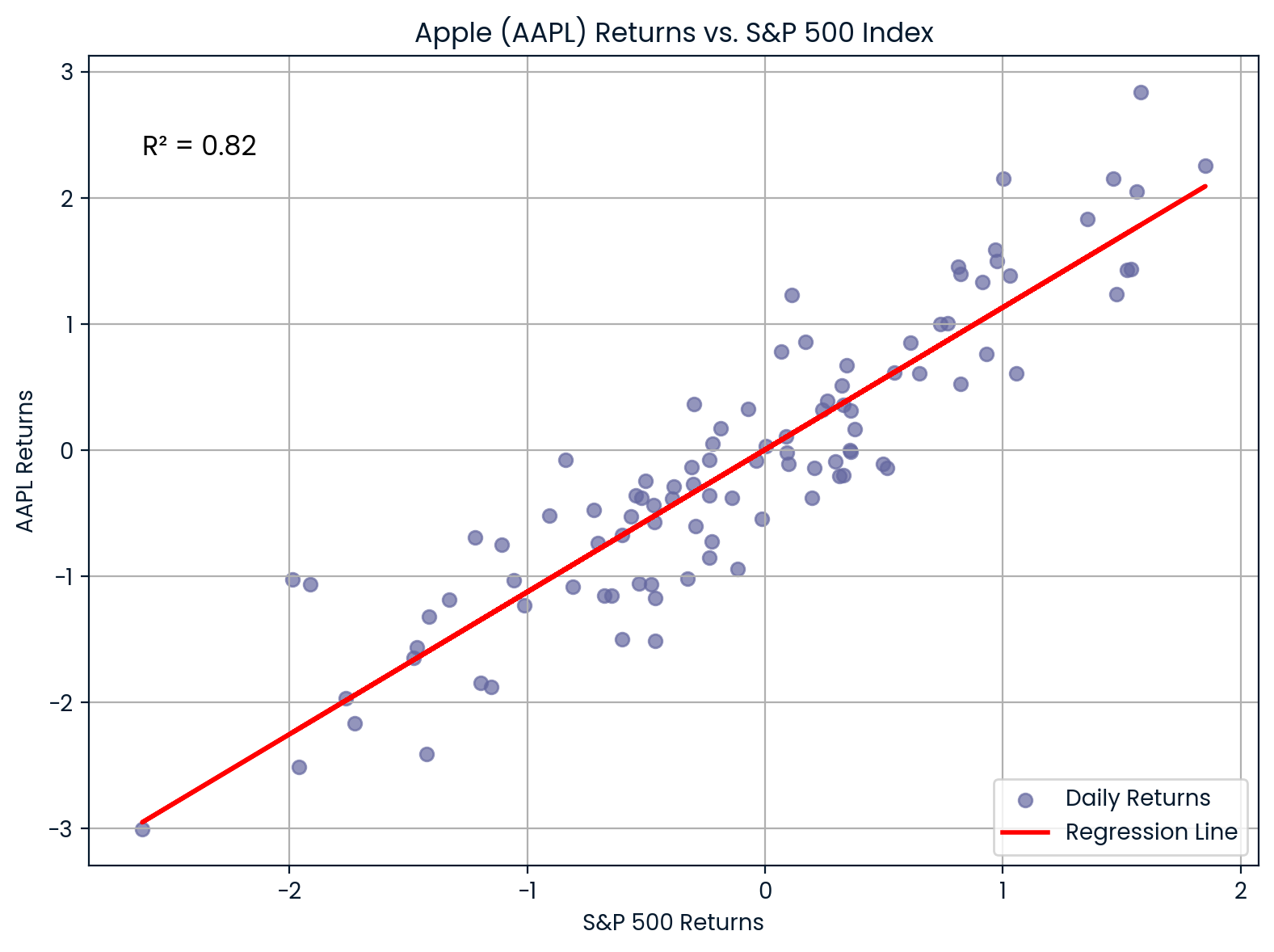
Correlation between AAPL and S&P 500. Image by Author.

The chart shows the strong correlation between Apple (AAPL) and the S&P 500. With an R^² of 0.82, most of Apple’s price movements align closely with market trends, indicating high market sensitivity.

Marketing: Ad spend and conversions

In marketing, R^² shows how well advertising spends explains customer conversion rates.

Suppose you work at an e-commerce company and want to know if increasing monthly ad spend improves conversion rates. You run a linear regression and find R^² = 0.98. That means 98% of the variation in conversion rate is explained by your ad spend, suggesting a very strong relationship.

These insights help marketers:

• Forecast conversion outcomes
• Justify ad budgets
• Predict return on investment (ROI)

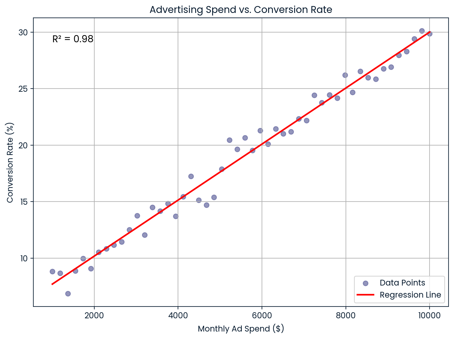
Monthly advertising spend vs conversion rate. Image by Author.

This chart illustrates a nearly perfect linear relationship between monthly advertising spend and conversion rate. It supports strong predictive value for ROI and budget planning.

Machine learning: Scoring regression models

In machine learning, R^² is used as a performance metric for regression tasks. Libraries like scikit-learn offer the r2_score() function to calculate it.

It tells you how well your model explains the variability in the data:

• R^² close to 1 means a good fit and low error

• R^² close to 0 means poor fit

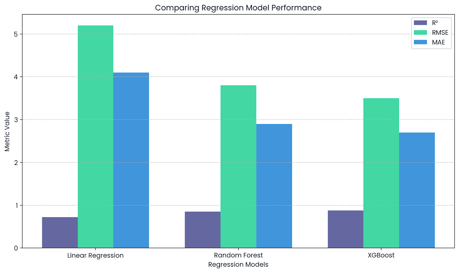
R^² complements RMSE and MAE. Image by Author.

This chart highlights how R² complements other metrics like RMSE and MAE when evaluating regression models. While R^² shows explanatory power, RMSE and MAE provide insights into the actual size of prediction errors.

Reporting The Coefficient of Determination in Research

If you're including R^² in a research paper or project, there are a few formatting rules you’ll want to keep in mind:

• Make sure you italicize R^² and yes, it should be a capital R, not lowercase. 
• Don’t use a leading zero before the decimal. So instead of writing R^² = 0.73, write R^² = .73. And unless you really need more detail, round it to two decimal places.

If you're using R^² as part of a regression analysis or ANOVA, and testing whether your model is significant, include a few more things: the F-statistic, degrees of freedom, and the p-value. These tell the reader how confident we can be that your model explains something meaningful.

So when you’re reporting results, it can look something like this:

“The model explained a significant portion of the variance in sales, R^² = .73, F(2, 97) = 25.42, p < .001.”

However, if you’re not conducting a hypothesis test, suppose you're performing exploratory analysis or evaluating a model's performance with cross-validation, then it’s perfectly fine to report the R² value on its own.

The Coefficient of Determination in Python, R, and Excel

Let’s see how to calculate R^² using three different ways: Python, R, and Excel through a mini-project where we predict student scores based on their study time.

We’ll use the following dataset for all three examples:

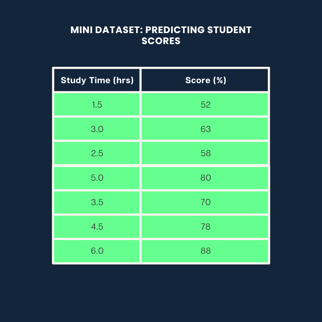
Example dataset. Image by Author

Coefficient of Determination in Python

Here’s how to calculate R^² in Python using scikit-learn:

from sklearn.linear_model import LinearRegression
from sklearn.metrics import r2_score
import numpy as np

# Data
study_time = np.array([1.5, 3.0, 2.5, 5.0, 3.5, 4.5, 6.0]).reshape(-1, 1)
scores = np.array([52, 63, 58, 80, 70, 78, 88])

# Model
model = LinearRegression()
model.fit(study_time, scores)
predicted_scores = model.predict(study_time)

# R² score
r2 = r2_score(scores, predicted_scores)
print(f"R² = {r2:.2f}")

0.99

This means 99% of the variance in scores is explained by study time.

If you want to learn more about Regression and stats models, you can check out our guide on Introduction to Regression with statsmodels in Python. 

Coefficient of Determination in R

In R, you can compute R² with a few lines using the lm() function:

# Data
study_time <- c(1.5, 3.0, 2.5, 5.0, 3.5, 4.5, 6.0)
scores <- c(52, 63, 58, 80, 70, 78, 88)

# Linear model
model <- lm(scores ~ study_time)

# R-squared
summary(model)$r.squared

0.9884718

About 98% of the variance in scores is explained by study time. If you want to learn more about Regression in R, check out our Introduction to Regression in R course.

Coefficient of Determination in Excel

In Excel, you can calculate R² using the built-in RSQ() function. Assuming:

• Study Time is in cells A2:A8

• Scores are in cells B2:B8

The syntax is:

RSQ(known_y's,known_x's)

I used the following formula:

=RSQ(B2:B8,A2:A8)

This tells Excel to compute the R^² value between the dependent variable (scores) and the independent variable (study time).

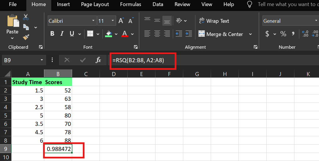
R^² example in Excel. Image by Author.  

Key Takeaways

Whether you’re predicting student scores, stock returns, or customer behavior, the coefficient of determination tells you how much of the outcome your model actually understands. 

A high coefficient of determination can look impressive, but don’t let it fool you into thinking the model is perfect or that it proves cause and effect. And a low coefficient of determination doesn’t always mean failure; it could mean your system is complex or your variables are incomplete.

So, if you're building or analyzing models, ask yourself:

• What am I explaining well?
• What am I missing?
• And is my model useful, not just accurate?

Start with that mindset, and you'll use the coefficient of determination as a lens for better decision-making.