Sensitivity and Specificity: A Complete Guide

Machine learning practitioners must evaluate both the quality of their data and the performance of their predictive models. 

Various metrics can help, especially when dealing with binary classification tasks; those where each data point is predicted to belong to one of two possible categories. Examples include credit approval (approve/don't approve), malware classification (malicious/not malicious), resume screening (shortlist/don’t shortlist), and disease diagnosis (has disease/doesn't have disease). Even A/B tests are closely related, essentially asking, "Is version B better than version A?" (yes/no).

Although accuracy provides a quick summary of performance, it can hide crucial information about the nature of a model's errors. For instance, a credit fraud detector labeling every transaction as legitimate might achieve 99% accuracy, yet completely fail to detect actual fraud. Sensitivity and specificity offer more nuanced insights, helping you understand not just how often a model is correct, but also what types of errors it makes and whether those errors are acceptable in context.

In this guide, you'll learn what sensitivity and specificity truly mean, when each metric is most appropriate, how they're calculated, and how to practically apply them in your work through clear, real-world examples.

Diagnostic testing and clinical decision making

Sensitivity and specificity originated in medical evaluation. Framing these metrics through the lens of diagnostic testing and clinical decision-making helps clarify many of the concepts in this article. To illustrate, we'll use two running examples, disease detection and credit card fraud.

• Diagnostic testing refers to a medical procedure used to confirm or exclude a disease.
• Assay testing measures whether a given substance is present in a sample. 
• Clinical decision-making is the process by which healthcare professionals gather information about a patient, consider diagnostic and treatment options, and make informed decisions based on evidence.

Target Audience

This article is for data practitioners who use statistical inference and want to understand metrics more nuanced than accuracy for better decision-making. These metrics help evaluate what types of errors a model makes and whether those errors are acceptable in context. Applications include medical diagnostics and fraud detection, as we have seen. Other applications include intrusion detection, quality control in manufacturing, and spam filtering.

Foundational Concepts of Sensitivity and Specificity

Before interpreting or applying sensitivity and specificity, it's essential to understand the basic concepts behind them. In this section, we discuss historic origins, core definitions, derivations, and calculations.

History

The concepts of sensitivity and specificity have their origins in biostatistics. Although used earlier in medical literature, biostatistics researcher Jacob Yerushlamy popularized the term in his paper "Statistical Problems in Assessing Methods of Medical Diagnosis, with Special Reference to X-Ray Techniques." 

In the 1970s, the receiver operating characteristic (ROC) curve (described later) became a tool to visually analyze sensitivity versus specificity in clinical testing. In the 1990s, machine learning adapted these concepts. Today, the terms are widely used in healthcare and machine learning for measuring how well systems identify true positives and true negatives.

Confusion Matrix

Suppose a machine learning model is used to detect fraudulent credit card transactions. Of a sample of 10,000 transactions, there are 9800 legitimate transactions and 200 cases of fraud. 

Since we're primarily interested in cases of fraud, let's designate fraudulent cases as positive, and non-fraudulent cases as negative. (Which cases are designated "positive" and "negative" are somewhat arbitrary; however, there is usually an obvious way to label the cases.) 

After running the model and comparing predicted fraud cases to actual fraud cases, we find that 160 fraud cases are correctly flagged, 9500 legitimate transactions are correctly identified, 300 legitimate transactions are incorrectly flagged as fraud, and 40 fraud cases are missed by the model.

To keep all this data straight, the following nomenclature is commonly used. 

• True positives (TP): 160 fraud cases are correctly flagged,
• True negatives (TN): 9500 legitimate transactions are correctly identified,
• False positives (FP): 300 legitimate transactions are incorrectly flagged as fraud, and
• False negatives (FN): 40 fraud cases are missed by the model.

The second letter (P or N) refers to whether the case was predicted to be positive or negative, and the first letter indicates whether or not that prediction was true (T) or false (F). 

So, a "false positive" indicates that the case was predicted to be positive, and that prediction was false, or in other words, the case was predicted to be positive, but was actually negative. Similarly, a false negative is a case that was predicted to be negative, but is actually positive.

To display this information, we commonly use a "confusion matrix," so called because it keeps track of how often the model confuses incorrect predictions with actual results (FN, FP). Here’s an example: 

Now, let's take a look at the row and column totals. The row sums indicate total predicted cases and the column sums indicate total actuals.

What do these totals represent?

• The first row total (460) represents the total number of predicted fraud cases (TP + FP).
• The second row total (9540) represents the total number of predicted legitimate cases (FN + TN).
• The first column total (200) represents the total number of actual fraud cases (TP + FN).
• The second column total (9800) represents the total number of actual legitimate cases (FP + TN)
• The grand total (10,000) equals the total size of our sample.

Definitions

Sensitivity (also known as true positive rate, or recall) measures the model's ability to correctly identify true positives. More precisely, sensitivity is the proportion of true positives to actual positives, TP / (TP + FN). 

Similarly, specificity (true negative rate) measures the model's ability to identify true negatives. It is the proportion of true negatives to actual negatives, TN / (FP + TN).

From a probabilistic point of view, sensitivity is the probability of a positive test given that the patient has the disease, and specificity is the probability of a negative test given that the patient does not have the disease.

Calculating Sensitivity and Specificity

In our fraud example, sensitivity = TP / (TP + FN) = 160/200, or 80%. Specificity is 9500/9800, or about 97%.

The Sensitivity-Specificity Trade-off and ROC Analysis

As model thresholds change, sensitivity and specificity often move in opposite directions. Increasing sensitivity typically reduces specificity, and vice versa. In this section, we explore this inherent trade-off and discuss how Receiver Operating Characteristic (ROC) analysis provides a visual and quantitative approach to evaluate model performance across various thresholds.

Trade-offs

Let's tweak the fraud example so that there are 20 more false negatives, FN = 60. Since the total number of actual fraud cases is still 200, there must now be 20 less true positives (TP = 140). 

Sensitivity has dropped from 80% to 140/200 = 70%. As the number of false negatives goes up, sensitivity goes down, and vice versa. This means that a high sensitivity indicates the number of false negatives is low.

In medical terms, a test with high specificity correctly identifies most people who do not have the condition. In our cancer screening example, a test with high specificity ensures that people who don't have cancer are not incorrectly told they do. 

This illustrates the trade-off between sensitivity and specificity. A few patients might be alarmed when told that they have cancer when they really don't, but people who truly do have the disease are correctly identified. In this case, high specificity is a better metric. In an imperfect world, we must make appropriate decisions based on an evaluation of trade-offs between metrics.

Threshold dynamics

A diagnostic threshold sets the cutoff value that determines if a test result is considered positive or negative. It converts a continuous value, such as a probability, into a yes/no cutoff. In everyday terms, it determines where to draw the line between positive or negative results.

The threshold is often set at 50%, or 0.50. A probability over 50% is considered positive, and one less than 50% is negative.

Changing the thresholds determines which cases are considered positive and negative. This shift affects the balance between catching true positives and avoiding false negatives. 

For instance, consider a model that outputs a probability of cancer. If the threshold is set at 0.3, the model classifies many people as positive. This approach works well for screening because it reduces the chance of missing cases. 

However, it increases the risk of false positives. If the threshold is 0.8, the model classifies fewer people as positive. This approach reduces false positives but increases the risk of missing actual cases.

When the threshold changes, the model shifts how often it catches true positives and how often it avoids false positives. Lower thresholds increase sensitivity but reduce specificity; higher thresholds reduce sensitivity but increase specificity. 

ROC curve interpretation

A Receiver Operating Characteristic (ROC) curve is a common visual to compare classification thresholds across values of sensitivity and specificity. The ROC curve plots sensitivity against 1 - specificity. Each point on the curve represents a specific threshold. As the threshold changes, the model's sensitivity and specificity adjust accordingly, tracing the ROC curve. 

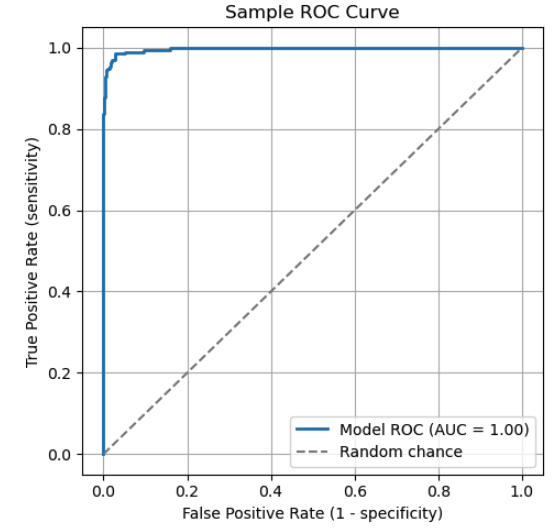
The ROC curve illustrates the trade-off between sensitivity and specificity. Key points on the curve: 

• (0,1): A perfect classifier that identifies all true positives without false negatives.
• (0,0): An extreme model that predicts everything as negative, misclassifying all positive cases.
• (1,1): An extreme model that predicts everything as positive, misclassifying all negative cases.

The diagonal dashed line represents random chance. A model that performs along this line has no real discriminative power. 

To evaluate a model using an ROC curve, consider the "Area Under the Curve" (AUC). The AUC is the total area (integral) under the curve, which represents a weighted average of performance across all thresholds. A higher AUC indicates better overall ability to distinguish between positive and negative classes.

Predictive Values and Likelihood Ratios

In this section, we explore how prevalence influences the reliability of test results. We also look at how likelihood ratios combine sensitivity and specificity into a single number that allows clinicians to update diagnostic probabilities after testing. 

Prevalence-dependent metrics

Positive Predictive Value (PPV), equivalent mathematically to precision in machine learning, reflects how likely a positive prediction is correct.. It measures the proportion of predicted positives that are true positives: PPV = TP / (TP + FP). 

Negative Predictive Value (NPV) reflects the reliability of a negative result. It measures the proportion of negative test results that are true negatives. Its formula is NPV = TN / (TN + FN).

Let's suppose we test 1000 people for an illness with this confusion matrix.

• PPV = TP / (TP + FP) = 80/100 = 80%.
• NPV = TN / (FN + TN) = 890 / 900 = 98.9%. 

For comparison, assume more people are ill (300 instead of 90), and adjust the confusion matrix accordingly.

As prevalence increases, the number of true positive cases rises. 

• Higher PPV. A positive result is now more likely to reflect actual illness. In fact, PPV = 270 / 300 = 90%, compared to 80% before, an increase of 10%.
• Lower NPV. A negative result becomes slightly less reliable, as there are more opportunities to miss true cases. We see NPV = 630 / 700 = 90%, which is a decrease of 8.9%.

Likelihood ratios

Likelihood ratios combine sensitivity and specificity into a single number that helps clinicians update their confidence in a diagnosis based on test results.

Probability versus odds

Before applying likelihood ratios, it's important to distinguish between probability and odds. Probability is the chance an event will occur, expressed by a value between 0 and 1. Odds represent how likely an event will happen relative to it not happening. 

A 75% probability means that the event occurs 75 times out of 100. The corresponding odds of the event are 0.75 / (1 - 0.75) = 0.75 / .025 = 3. This means the odds are 3 to 1 in favor of the event happening.

More generally, if p is the probability of an event, then odds = p / (1 - p). Converting from odds to probability, p = odds / (1 + odds).

Likelihood ratios

The positive likelihood ratio (LR+) tells you how much a positive result increases the odds of having the condition compared to someone without it. Higher values (>10) suggest the test is very effective at ruling in the condition. The formula is LR+ = Sensitivity / (1 - Specificity). 

The negative likelihood ratio (LR-) tells you how much a negative result decreases the odds of having the condition compared to someone without it. Lower values (< 0.1) suggest the test is very effective at ruling out a condition. The formula is LR- = (1 - Sensitivity) / Specificity.

Post-test probability

To make decisions, clinicians begin with a pre-test probability estimated on factors such as the patient's symptoms and history. This estimate is combined with the likelihood ratio to calculate the post-test probability.

The procedure is as follows.

1. Start with a pre-test probability p.
2. Convert to odds. Pre-test odds = p / (1 - p).
3. Apply the likelihood ratio. If the test is positive, multiply the pre-test odds by LR+, if negative, multiply by LR-. Post-test odds = pre-test odds x LR.
4. Convert post-test odds back to probability. Post-test probability = Post-test odds / (1 + post-test odds).

For example, suppose the pre-test probability of disease is 30% and LR+ = 10. What is the post-test probability? 

1. p = 0.3
2. Pre-test odds = 0.3/0.7 = 0.43. 
3. Post-test odds = 0.43 * 10 = 4.3
4. Post-test probability = 4.3 / (1 + 4.3) = 81%.

We see that LR+ significantly shifted the probability and the confidence in a diagnosis.

Advanced Methodologies and Future Directions

As diagnostic testing and classification systems become more complex, new methodologies are emerging to push beyond traditional performance limits. In this section, we explore how Bayesian approaches enable personalized decision thresholds and how novel technologies like CRISPR-based diagnostics are pushing the frontiers of analytical sensitivity and specificity.

Bayesian approaches

The idea of starting with a prior belief and updating it based on new information lies at the core of Bayesian statistics. It provides a formal way to revise probabilities in the light of new data. 

Bayesian reasoning relies on three key components.

• Prior probability. This is the initial belief before seeing new evidence. ("The forecast said there is a 60% risk of rain.")
• The likelihood. This is how likely the new evidence is if the belief is correct.  ("I heard rain, so the likelihood of a correct forecast is high.")
• Posterior probability. This is the revised belief after considering new evidence. It is found by multiplying the prior probability by the likelihood. 

This is described mathematically by Bayes theorem.

P(A|B) = P(B|A) x P(A) / P(B)

where P(A|B) is the posterior (the probability of A given B), P(B|A) is the likelihood (the probability of B given that A is true), P(A) is the prior, and P(B) is the evidence.

Optimizing thresholds with Bayesian approaches

As we've seen, traditional classification models often apply a fixed threshold, such as 0.5, to determine if an output should be labeled positive or negative. Bayesian approaches, by contrast, allow these thresholds to adapt based on context, including individual risk factors, demographics, behavior history, or real-time data. This flexibility enables systems to adjust thresholds dynamically, rather than relying on a one-size-fits-all static threshold.

Consider a model that predicts the likelihood of heart disease. A traditional model might use a threshold of 0.5. Patients with a probability over 50% are considered positive, and those below as negative.

Now, consider a Bayesian approach with two hypothetical patients:

• Patient A is a 68-year-old lifelong smoker with a family history of heart disease and recent chest pain.
• Patient B is a 25-year-old non-smoker with no symptoms or relevant history.

Both patients receive a test-generated probability of 0.45. A fixed threshold model with a threshold of 0.5 would treat both of these patients as negative. 

However, a Bayesian model incorporates prior risk information and may be used along with prediction intervals. For patient A, the system may lower the decision threshold, flagging the case for further evaluation. For patient B, it may keep the threshold, and no follow-up is recommended.

In this way, Bayesian methods tailor the classification threshold to each patient's context, leading to more clinically appropriate decisions.

High-sensitivity/specificity assays

An emerging technology that pushes the limits of analytical sensitivity and specificity is CRISPR-Based diagnostics. Scientists adapted CRISPR (Clustered Regularly Interspaced Short Palindromic Repeats), a gene-editing tool, to detect genetic material. It utilizes Cas proteins to detect specific nucleic acid sequences with high sensitivity.

CRISPR-based assays have been used for the early detection of cancer. Portable cancer diagnostic tools are being developed for use in clinical settings. Two important diagnostic platforms are SHERLOCK and DETECTR. 

CRISPR-based assays offer many advantages. They provide high sensitivity, so they can detect minute quantities of DNA or RNA. 

This makes them valuable for identifying early-stage infections, cancer, or rare mutations. They also offer exceptional specificity, allowing them to distinguish between closely related genetic sequences to reduce false positives. Additional benefits include rapid results and low-cost, portable equipment. 

These assays support a wide range of applications, including infectious disease detection, cancer diagnostics, and genetic disease screening. Researchers can use machine learning to optimize guide RNA design and improve diagnostic accuracy.

CRISPR-based assays also face challenges. Most only provide a binary result (positive or negative). Standardization and reproducibility remain concerns, as results vary across laboratories and testing conditions. 

Additionally, these assays must meet regulatory requirements, including FDA and CLIA approval, which require extensive validation, documentation, and review. Finally, IP issues complicate licensing and slow down commercialization.

Conclusion

Sensitivity and specificity play a central role in evaluating diagnostic tests and classification models. They can be more insightful than accuracy, especially in imbalanced data sets or when false positives or false negatives carry different costs. Along with related tools such as likelihood ratios and ROC analysis, they guide insightful interpretation and better decision making.

Want to deepen your practical skills in evaluating model performance? Be sure to explore these DataCamp resources:

• Machine Learning Fundamentals in Python: Learn foundational concepts and techniques.
• Model Validation in Python: Gain hands-on experience with sensitivity, specificity, ROC curves, and more.
• Biomedical Image Analysis in Python: Apply these concepts directly in healthcare diagnostics scenarios.