Policy Gradient Theorem Explained: A Hands-On Introduction

Why Use Policy Gradient Methods?

One key advantage of policy gradient methods is their ability to handle complex action spaces, where traditional value-based approaches struggle.

Handling high-dimensional action spaces

Value-based methods, such as Q-learning, work by estimating the value function for all possible actions. This becomes difficult when the environment’s action space is either continuous or discrete but large. 

Policy gradient methods parametrize the policy and estimate the gradient of the cumulative rewards with respect to the policy parameters. They use this gradient to directly optimize the policy by updating its parameters. Hence, they can efficiently handle high-dimensional or continuous action spaces. Policy gradients are also the basis of Reinforcement Learning using Human Feedback (RLHF) methods. 

By parameterizing the policy and adjusting its parameters based on gradients, policy gradients can efficiently handle continuous and high-dimensional actions. This direct approach enables better generalization and more flexible exploration, making it well-suited for tasks like robotic control and other complex environments.

Learning stochastic policies

Given a set of observations: 

• A deterministic policy specifies what action the agent takes. 
• A stochastic policy gives a set of actions and the probability of the agent choosing each action. 

When following a stochastic policy, the same observation can lead to choosing different actions in different iterations. This promotes exploration of the action space and prevents the policy from getting stuck in local optima. Because of this, stochastic policies are useful in environments where exploration is essential to discovering the path that leads to the maximum returns. 

In policy-based methods, the policy output is converted into a probability distribution, with each possible action assigned a probability. The agent chooses an action by sampling this distribution, making it possible to implement a stochastic policy. Thus, policy gradient methods combine exploration with exploitation, useful in environments with complex reward structures. 

Derivation of the Policy Gradient Theorem

Before diving into the derivation, it’s important to establish the mathematical notation and key concepts used throughout the proof.

Mathematical notation and preliminaries

As mentioned in a previous section, the policy gradient theorem states that the derivative of the expected return is the expectation of the product of the return and the derivative of the logarithm of the policy. 

Before deriving the policy gradient theorem, we introduce the notation:

• E[X] refers to the probabilistic expectation of a random variable X. 
• Mathematically, the policy is expressed as a probability matrix that gives the probability of choosing different actions based on different observations. A policy is typically modeled as a parametrized function, with the parameters represented as θ.
• π_θ refers to a policy parametrized by θ. In practice, these parameters are the weights of the neural network that models the policy. 
• The trajectory, τ, refers to a sequence of states, typically starting from a randomized initial state till either the current timestep or the terminal state. 
• ∇_θf refers to the gradient of a function f with respect to parameter(s) θ. 
• J(π_θ) refers to the expected return achieved by the agent following the policy π_θ. This is also the objective function for gradient ascent. 
• The environment gives a reward at each timestep, depending on the agent’s action. The return refers to the cumulative rewards from the initial state to the current timestep. 
• R(τ) refers to the return generated over the trajectory τ. 

Derivation steps

We show how to derive and prove the policy gradient theorem from first principles, starting with the expansion of the objective function and using the log-derivative trick. 

The objective function (Equation 1)

The objective function in the policy gradient method is the return 

J accumulated by following the trajectory based on the policy π expressed in terms of parameters θ. This objective function is given as: 

In the above equation: 

• The left-hand side (LHS) is the expected return achieved by following the policy π_θ.
• The right-hand side (RHS) is the expectation (over the trajectory τ generated by following the policy π_θ in each step) of the returns R(τ) generated over the trajectory τ.  

The differential of the objective function (Equation 2)

Differentiating (with respect to θ) both sides of the above equation gives:

The gradient of the expectation (Equation 3)

The expectation (on the RHS) can be expressed as an integral over the product of: 

• The probability of following a trajectory τ
• The returns generated over the trajectory τ

Thus, the RHS of Equation 2 is restated as: 

The gradient of an integral is equal to the integral of the gradient. So, in the above expression, we can bring the gradient ∇_θ under the integral sign. So, the RHS becomes: 

Thus, Equation 2 can be re-written as:

The probability of the trajectory (Equation 4)

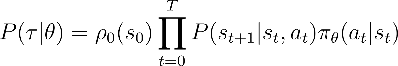
We now take a closer look at P(τ|θ), the probability of the agent following trajectory τ given policy parameters θ (and hence policy π_θ). A trajectory consists of a set of steps. Thus: 

• The probability of obtaining trajectory τ is the product of:
• The probability of following all the individual steps. 

• In the time step t, the agent goes from state s to state s_t+1 by following action a_t. The probability of this happening is given the product of:
• The probability of the policy predicting action a_t in state s_t
• The probability of ending up in state s_t+1 given action a_t and state s_t

Thus, starting from an initial state s₀, the probability of the agent following trajectory τ based on policy π_θ is given as: 

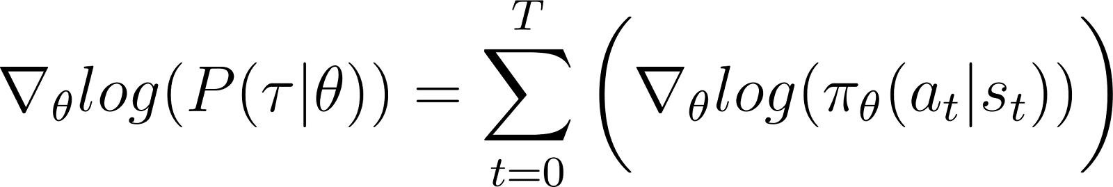
To make things simpler, we want to express the product in the RHS above as a sum. So, we take  the logarithm on both sides of the above equation:

The derivative of the log-probability (Equation 5) 

We now take the derivative (with respect to θ) of the log probability in the above equation. 

On the RHS of the above equation: 

• The first term log ρ₀(s₀) is constant with respect to θ. So its derivative is 0. 
• The first term inside the summation P(s_t+1|s_t, a_t) is also independent of θ and its derivative with respect to θ is also 0. 

Removing the above zero-terms from the equation, we are left with (Equation 5): 

Recall from Equation 2 that: 

Equation 5 evaluates the log of the first part of the RHS of Equation 2. We need to relate the derivative of a term with its logarithm. We do this using the chain rule and the log-derivative trick. 

The log-derivative trick

We take a detour and use the rules of calculus to derive a result, which we will use to simplify the previous equation and render it suitable for computational methods. 

In calculus, the derivative of a logarithm can be expressed as: 

Thus, by re-arranging the above equation, the derivative of x can be expressed in terms of the derivative of the logarithm of x:

This is sometimes called the log-derivative trick. 

The chain rule

According to the chain rule, given z(y) as a function of y, where y itself is a function of θ, y(θ), the derivate of z with respect to θ is given as:

In this case, y(θ) stands for P(θ) and z(y) stands for log(y). Thus, 

Applying the chain rule

We know from calculus that d(log(y)) / dy = 1/y. Use this in the first expression of the RHS above. 

Move y to the LHS and use the notation:

y stands for P(θ). So the above equation is equivalent to: 

Applying the log-derivative trick

The above result gives the first expression of the RHS of Equation 2 (shown below).  

Using the result in the RHS of Equation 2, we get: 

We rearrange the terms under the RHS integral as below:

Deriving the final result

Observe that the above expression contains the integral expansion of an expectation: ∫P(θ)∇logP(θ) = E[∇logP(θ)]

Thus, the RHS above can be expressed as the expectation: 

We substitute the derivative of the log probability in the expression of the expected reward: 

In the above equation, substitute the value of ∇logP(θ) from Equation 5 to get: 

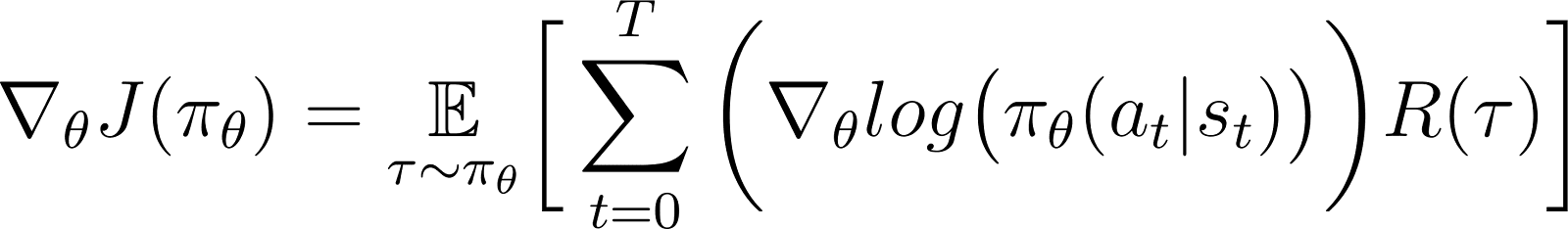
This is the expression for the gradient of the reward function according to the policy gradient theorem. 

The intuition behind the policy gradient

Policy gradient methods convert the policy’s output to a probability distribution. The agent samples this distribution to pick an action. Policy gradient methods adjust the policy parameters. This leads to updating this probability distribution in each iteration. The updated probability distribution has a higher likelihood of choosing actions that lead to higher rewards. 

The policy gradient algorithm computes the gradient of the expected return with respect to the policy parameters. By moving the policy parameters in the direction of this gradient, the agent increases the probability of choosing actions that result in higher rewards during training. 

Essentially, actions that led to better outcomes become more likely to be chosen in the future, gradually improving the policy to maximize long-term rewards.

Implementing Policy Gradients in Python

Having discussed the fundamental principles of policy gradients, we show how to implement them using PyTorch and Gymnasium. 

Setting up the environment

As a first step, we need to install gymnasium and a few supporting libraries like NumPy and PyTorch.

To install gymnasium and its dependencies on a server or local machine, run:

$ pip install gymnasium 

To install using a Notebook like Google Colab or DataLab, use: 

!pip install gymnasium

You import these packages within the Python environment:

import torch
import torch.nn as nn
import torch.optim as optim
import torch.nn.functional as F
import torch.distributions as distributions
import numpy as np
import gymnasium as gym  

Coding a simple policy gradient agent

Create an instance of the environment using the .make() method.

env = gym.make('CartPole-v1')

As with other machine learning methods, we use a neural network to implement the policy gradient agent. 

CartPole-v1 is a simple environment, so we design a simple network with 1 hidden layer with 64 neurons. The input layer’s dimension equals the dimensions of the observation space. The output layer’s dimension equals the size of the environment's action space. Thus, the policy network maps observed states to actions. Given an observation as input, the network outputs the predicted action according to the policy. 

The code below implements the policy network: 

class PolicyNetwork(nn.Module):
    def __init__(self, input_dim, hidden_dim, output_dim, dropout):
        super().__init__()

        self.layer1 = nn.Linear(input_dim, hidden_dim)
        self.layer2 = nn.Linear(hidden_dim, output_dim)
        self.dropout = nn.Dropout(dropout)

    def forward(self, x):
        x = self.layer1(x)
        x = self.dropout(x)
        x = F.relu(x)
        x = self.layer2(x)
        return x

Training the agent

The environment gives a reward in each timestep depending on the agent’s state and action. The policy gradient approach consists of running gradient descent on the cumulative rewards (return). The goal is to maximize the total return. 

To calculate the return in an episode, you accumulate (with a discount factor) rewards from all the timesteps in that episode. Additionally, normalizing the returns is helpful to ensure smooth and stable training. The code below shows how to do this:

def calculate_stepwise_returns(rewards, discount_factor):
    returns = []
    R = 0

    for r in reversed(rewards):
        R = r + R * discount_factor
        returns.insert(0, R)
    returns = torch.tensor(returns)
    normalized_returns = (returns - returns.mean()) / returns.std()
    return normalized_returns

In each iteration of the forward pass, we do the following steps: 

• Run the agent based on the current policy using the .step() function. The policy predicts the probability of taking the chosen action in each timestep.
• Receive the reward from the environment based on the agent’s action.
• Accumulate stepwise rewards and the log probabilities of the actions until the agent reaches a terminal state.

The code below implements the forward pass:

def forward_pass(env, policy, discount_factor):
    log_prob_actions = []
    rewards = []
    done = False
    episode_return = 0

    policy.train()
    observation, info = env.reset()

    while not done:
        observation = torch.FloatTensor(observation).unsqueeze(0)
        action_pred = policy(observation)
        action_prob = F.softmax(action_pred, dim = -1)
        dist = distributions.Categorical(action_prob)
        action = dist.sample()
        log_prob_action = dist.log_prob(action)

        observation, reward, terminated, truncated, info = env.step(action.item())
        done = terminated or truncated

        log_prob_actions.append(log_prob_action)
        rewards.append(reward)
        episode_return += reward

    log_prob_actions = torch.cat(log_prob_actions)
    stepwise_returns = calculate_stepwise_returns(rewards, discount_factor)

    return episode_return, stepwise_returns, log_prob_actions

Using backpropagation and gradient ascent to update the policy

In traditional machine learning:

• Loss refers to the difference between the predicted and the actual output. 
• We minimize the loss using gradient descent.

In RL:

• The loss is a proxy for the quantity on which gradient descent (or ascent) is to be applied. 
• We maximize the return (cumulative rewards) using gradient ascent.
• The expected return value is used as a proxy for the loss for gradient descent. The expected return value is the product of:
• The returns expected from each step with 
• The probability of choosing the sampled action in each step. 
• To apply gradient ascent using backpropagation, we use the negative of the loss. 

The code below calculates the loss:

def calculate_loss(stepwise_returns, log_prob_actions):
    loss = -(stepwise_returns * log_prob_actions).sum()
    return loss

Similar to standard machine learning algorithms, to update the policy, you run backpropagation with respect to the loss function. The update_policy() method below invokes the calculate_loss() method. It then runs backpropagation on this loss to update the policy parameters, i.e., model weights of the policy network. 

def update_policy(stepwise_returns, log_prob_actions, optimizer):
    stepwise_returns = stepwise_returns.detach()
    loss = calculate_loss(stepwise_returns, log_prob_actions)
    
    optimizer.zero_grad()
    loss.backward()
    optimizer.step()

    return loss.item()

The training loop 

We use the functions defined earlier to train the policy. Before starting the training, we need: 

• An untrained policy initialized as a randomized instance of the PolicyNetwork class. 
• An optimizer that uses the Adam algorithm. 
• Hyperparameters for the discount factor, learning rate, dropout rate, reward threshold, and the maximum number of training epochs. 

We iterate through the training loop until the average return exceeds the reward threshold. In each iteration, we execute the following steps: 

• For each episode, run the forward pass once. Collect the log probability of actions, the stepwise returns, and the total return from that episode. Accumulate the episodic returns in an array. 
• Calculate the loss using the log probabilities and the stepwise returns. Run the backpropagation on the loss. Use the optimizer to update the policy parameters. 
• Check if the average return over N_TRIALS exceeds the reward threshold. 

The code below implements these steps:

def main(): 
    MAX_EPOCHS = 500
    DISCOUNT_FACTOR = 0.99
    N_TRIALS = 25
    REWARD_THRESHOLD = 475
    PRINT_INTERVAL = 10
    INPUT_DIM = env.observation_space.shape[0]
    HIDDEN_DIM = 128
    OUTPUT_DIM = env.action_space.n
    DROPOUT = 0.5

    episode_returns = []

    policy = PolicyNetwork(INPUT_DIM, HIDDEN_DIM, OUTPUT_DIM, DROPOUT)

    LEARNING_RATE = 0.01
    optimizer = optim.Adam(policy.parameters(), lr = LEARNING_RATE)

    for episode in range(1, MAX_EPOCHS+1):
        episode_return, stepwise_returns, log_prob_actions = forward_pass(env, policy, DISCOUNT_FACTOR)
        _ = update_policy(stepwise_returns, log_prob_actions, optimizer)

        episode_returns.append(episode_return)
        mean_episode_return = np.mean(episode_returns[-N_TRIALS:])

        if episode % PRINT_INTERVAL == 0:
            print(f'| Episode: {episode:3} | Mean Rewards: {mean_episode_return:5.1f} |')

        if mean_episode_return >= REWARD_THRESHOLD:
            print(f'Reached reward threshold in {episode} episodes')
            break

Run the training program by calling the main() function:

main()

This DataLab workbook contains the above implementation of the policy gradient algorithm. You can run it directly or use it as a starting point for modifying the algorithm.

Advantages and Challenges of Policy Gradient Methods

Policy gradient methods offer several advantages, such as:

• Handling continuous action spaces: Value-based methods (like Q-learning) are inefficient with continuous action spaces because they need to estimate values over the entire action space. Policy gradient methods can directly optimize the policy using the gradient of the expected returns. This approach works well with continuous action distributions. Thus, policy gradient methods are suitable for tasks like robotic control which are based on continuous action spaces.
• Stochastic policies: Policy gradient methods can learn stochastic policies - which give a probability of selecting each possible action. This allows the agent to try a variety of actions and reduces the risk of getting stuck in local optima. It helps in complex environments where the agent needs to explore the action space to find the optimal policy. The stochastic nature helps balance exploration (trying new actions) and exploitation (choosing the best-known actions), which is crucial for environments with uncertainty or sparse rewards.
• Direct policy optimization: Policy gradients optimize the policy directly instead of using value functions. In continuous or high-dimensional action spaces, approximating values for every action can become computationally expensive. Thus, policy-based methods perform well in such environments. 

Notwithstanding their many advantages, policy gradient methods have some inherent challenges:

• High variance in gradient estimates: Policy gradient methods select actions by sampling a probability distribution. In effect, they sample the trajectory to estimate the expected return. Because the sampling process is inherently random, the estimated returns in subsequent iterations can have high variance. This can make it difficult for the agent to learn efficiently because the updates to the policy may fluctuate significantly between iterations. 
• Instability during training: 
• Policy gradient methods are sensitive to hyperparameters like the. If the learning rate is too high, the updates to the policy parameters can be too large, causing the training to miss the optimum parameters. On the other hand, if the learning rate is too small, convergence can be slow. 
• Policy gradient methods need to balance exploration and exploitation. If the agent does not explore enough, it may not reach the neighborhood of the optimal policy. Conversely, if it explores too much, it will not converge on the optimal policy and oscillate around the action space. 
• Sample inefficiency: Policy gradient methods estimate the return by following through with each policy till termination and accumulating the rewards from each step. Thus, they need many interactions with the environment to draw a large number of sample trajectories. This is inefficient and expensive for environments with large state or action spaces. 

Solutions for stability

Since instability is a relatively common problem in policy gradient methods, developers have adopted various solutions to stabilize the training process. Below, we introduce common solutions for stabilizing training using policy gradients: 

Using baseline functions

Due to inefficient sampling, the gradients of the returns estimated during the training iterations can have high variance, making the training unstable and slow. A common approach to reducing the variance is to use baseline functions, such as the Advantage Actor-Critic (A2C) method. The idea is to use a proxy (the advantage function) instead of the estimated return for the objective function. 

The advantage is calculated as the difference between the actual return from the sampled trajectory and the expected return given the initial state. This approach involves using the value function as the expected value of states and state-action pairs. By representing the loss as the difference between the actual return and the expected return instead of as the returns alone, A2C reduces the variance in the loss function and, hence, in the gradients, making the training more stable. 

Using entropy regularization

In certain environments, such as those with sparse rewards (only very few states give a reward), the policy quickly adopts a deterministic approach. It also adopts a greedy approach and exploits the paths it has already explored. This prevents further exploration and often leads to convergence to local optima and suboptimal policies. 

The solution is to encourage exploration about penalizing the policy when it becomes too deterministic. This is done by adding an entropy-based term to the objective function. The entropy measures the amount of randomness in the policy. The greater the entropy, the more randomness in the actions chosen by the agent. This entropy-based term is the product of the entropy coefficient and the entropy of the current policy. 

Making the entropy a part of the objective function helps to achieve a balance between exploitation and exploration. 

Policy Gradient Extensions

Among the various extensions of policy gradient methods, one of the most fundamental is the REINFORCE algorithm. It provides a straightforward implementation of the policy gradient theorem and is the foundation for more advanced techniques.

REINFORCE algorithm

The REINFORCE algorithm, also known as Monte Carlo Reinforce, is one of the basic implementations of the policy gradient theorem. It uses Monte Carlo methods to estimate returns and policy gradients. When following the REINFORCE algorithm, the agent directly samples all the actions (from the initial to the terminal state) from the environment. This contrasts with other methods like TD-Learning and Dynamic Programming, which bootstrap their actions based on value function estimates. 

Below, we present the basic steps of the REINFORCE algorithm:

• Initialize the policy with random parameters
• Repeat multiple training episodes. For each episode: 
• Generate each step of the entire episode as follows: 
• Pass the state to the policy function. 
• The policy function generates probabilities for each possible action.
• Randomly sample an action from this probability distribution.
• For each state in the episode, estimate the returns (discounted cumulative rewards) until step.
• Estimate the gradient of the objective function (according to the policy gradient theorem), expressed as the product of the stepwise returns and the action probabilities for each step. 
• Update the policy parameters by applying the gradients

For each policy, you can sample a single trajectory to estimate the gradient (as shown above) or average the gradient over multiple trajectories sampled under the same policy. 

Actor-critic methods

Actor-critic methods combine policy gradient methods (like REINFORCE) with value functions.

• The actor's workings are similar to policy gradient methods. The actor implements the policy, selecting actions in each step based on the policy. It updates the policy by following the gradient of the expected return. 
• The critic implements the value function, which is used as a baseline (discussed in the previous section). This helps to make the training more efficient and stable. 

Policy gradient methods like REINFORCE estimate the gradients along each trajectory using the raw return. Because a sampling process draws these trajectories, it can lead to large variances in the returns and gradients. Using an advantage function instead of the raw returns solves this problem. The advantage function is the difference between the actual and expected returns (i.e., the value function). Actor-critic methods are a class of algorithms. When the critic is implemented using the advantage function (the most common approach), it is also called Advantage actor-critic (A2C). 

Proximal Policy Optimization (PPO)

In complex environments, actor-critic methods like A2C alone are not sufficient to control the variance in the returns and gradients. In such cases, artificially restricting the amount by which the policy can change in each iteration helps. This forces the updated (after gradient ascent) policy to lie in the neighborhood of the old policy. 

Methods like Proximal Policy Optimization make two modifications to policy gradients:

• Use an advantage function. Typically, this advantage function uses the value function as the baseline. In this, they are similar to A2C methods. 
• Restrict the amount by which the policy parameters can change in each iteration. This is done using a clipped surrogate objective function. The algorithm specifies a range within which the ratio of the new policy to the old policy must lie. When the ratio (after gradient update) exceeds these predetermined values, it is clipped to lie within the range. 

Thus, PPO significantly improves vanilla policy gradient methods, which improves stability in complex environments. The clipped objective function prevents large variances in the returns and gradients from destabilizing the policy updates. To achieve a balance between exploration and exploitation, it is also possible to modify PPO to use entropy regularization. This is done by adding an entropy term (a scaling parameter multiplied by the entropy of the policy) to the objective function. 

Recent advances

Policy gradients are among the earliest methods used to solve RL problems. After the advent of fast GPUs, various new approaches have been proposed to apply modern ML techniques to policy gradients. 

Gradient-Boosted Reinforcement Learning 

In recent years, progress has been made in applying methods like gradient boosting to RL algorithms. Gradient boosting combines the predictions from multiple weak models to generate a single strong model. This is referred to as Gradient-Boosted Reinforcement Learning (GBRL). GBRL is a Python package similar to XGBoost that implements these techniques for RL algorithms.

Transfer Reinforcement Learning 

Transfer learning (TL) is a technique where the knowledge acquired by one model is applied to improve the performance of another model. Transfer learning is helpful because training ML models from scratch is expensive. TL approaches have been used with policy gradients to improve the performance of RL models. This approach is called Transfer Reinforcement Learning (TRL). 

Conclusion

Policy gradients are among the most fundamental approaches to solving RL problems.

 In this article, we presented the first principles of policy gradients and showed how to derive the policy gradient theorem. We also demonstrated how to implement a simple gradient-based algorithm using PyTorch in a Gymnasium environment. Lastly, we discussed practical challenges and common extensions to the basic policy gradient algorithm.

If you want to deepen your understanding of reinforcement learning and deep learning with PyTorch, check out these courses:

• Reinforcement Learning Track – Learn the foundations of RL, from value-based methods to policy optimization techniques.
• Introduction to Deep Learning with PyTorch – Get hands-on experience with PyTorch and build deep learning models from scratch.