Random Forest Regression: A Complete Guide

What Is Random Forest Regression?

Random forest regression is an ensemble technique that builds multiple randomized decision trees and combines their outputs to produce a continuous prediction. Instead of relying on a single model, it aggregates predictions from many trees, typically by taking the average of their outputs.

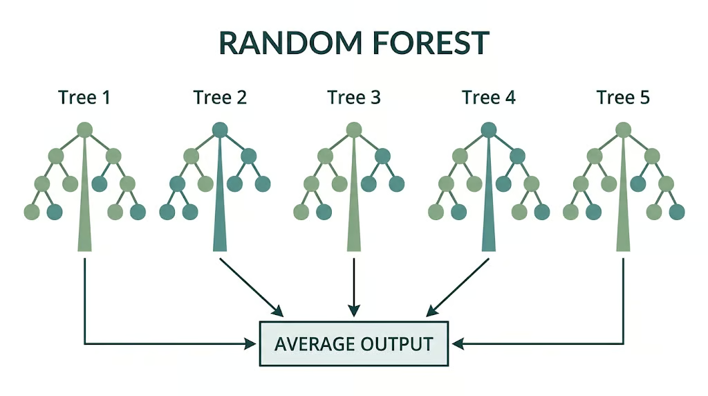
Why multiple trees? A single decision tree tends to overfit. It captures noise along with signals, especially when working with messy, real-world data.

Bootstrap aggregating and feature randomness

The strength of the Random Forest Regression model comes from how it introduces randomness at each step and then aggregates results to reduce variance. Let’s discuss this internal mechanism. 

Bootstrap aggregating, or bagging, trains each tree on a different random subset of the data. This introduces variation across trees and reduces the risk of overfitting. 

Feature randomness adds another layer of diversity by selecting a random subset of features at each split. Together, these techniques stabilize predictions and improve generalization.

Bootstrap sampling and feature randomness

Random Forest starts with bootstrap sampling, also known as bagging. Each tree is trained on a randomly sampled subset of the original dataset. As a result, the trees learn different patterns instead of repeating the same structure.

It also introduces feature randomness. At each split, the model considers only a random subset of features instead of all available ones. This prevents a few dominant features from controlling every tree. 

Together, bagging and feature randomness create a set of uncorrelated trees that make different errors, so when combined, their predictions cancel out noise and improve overall accuracy.

Growing trees and aggregating predictions

Each tree in the forest grows deep, often without pruning. This allows the model to capture complex patterns, interactions, and non-linear relationships in the data. 

These individual trees may overfit, but that effect is reduced when Random Forest aggregates their outputs for the final result.

The bias-variance trade-off

Random forest balances two key factors: the strength of individual trees and the diversity of the forest. 

Deep trees have low bias because they can closely fit the training data. At the same time, randomness in data sampling and feature selection reduces correlation between trees. By averaging many low-bias, weakly correlated trees, the model reduces overall variance without increasing bias.

Data Preprocessing and Implementation Workflow

Next, we’ll put the concepts into practice and look at techniques for turning raw data into a working Random Forest model.

Data cleaning and feature engineering

Data preparation for Random Forest models usually starts with handling categorical variables. 

• For smaller categories, one-hot encoding works well and is reliable
• For high-cardinality features, target encoding is often more efficient, as it captures category-level signals without significantly increasing dimensionality

Next comes missing data. The approach depends on the library you are using. Some implementations can handle missing values directly during splits, while others expect you to fill them in. In most cases, simple imputation using median or mode is enough. Since Random Forest does not rely on strict distributions, these straightforward methods hold up well in practice.

After all, the bigger impact comes from feature engineering. For example, lag variables introduce temporal dependencies, rolling aggregates capture local trends, and grouped statistics encode higher-level patterns. These engineered features allow the model to better represent information and improve predictive performance.

For a deeper look, I recommend reading my Feature Engineering in Machine Learning tutorial.

Establishing baselines and splitting strategies

Before tuning anything, the first step is to split the data correctly. 

For standard tabular problems, that usually means separating the dataset into train, validation, and test sets so the model is trained on one slice, tuned on another, and evaluated on a final untouched slice. 

That separation matters because it gives you a realistic read on how the model will behave on new data.

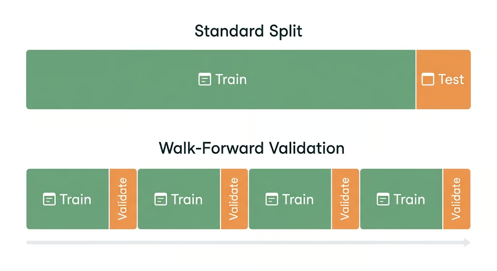
For time series, the splitting strategy changes. Random splits can leak future information into the past, which makes performance look better than it really is.

Walk-forward validation avoids that problem by training on an initial time window, validating on the next window, then moving forward step by step. That keeps the evaluation aligned with the way the model would actually be used in production.

Writing the end-to-end Python implementation

The implementation follows a simple scikit-learn flow: 

1. Import the model
2. Split the data
3. Fit the estimator
4. Generate predictions
5. Evaluate the output

A typical setup looks like this in practice:

from sklearn.ensemble import RandomForestRegressor
from sklearn.model_selection import train_test_split
from sklearn.metrics import mean_absolute_error, root_mean_squared_error
import matplotlib.pyplot as plt

X_train, X_test, y_train, y_test = train_test_split(
    X, y, test_size=0.2, random_state=42
)

model = RandomForestRegressor(random_state=42)
model.fit(X_train, y_train)

y_pred = model.predict(X_test)

mae = mean_absolute_error(y_test, y_pred)
rmse = root_mean_squared_error(y_test, y_pred)

Once the model is trained and evaluated, the next step is to visualize predicted values against actual values. 

A scatter plot makes it easy to spot systematic bias, such as predictions that consistently overshoot or undershoot the target. It also helps reveal heteroscedasticity, where prediction errors widen as the target values increase.

Hyperparameter Tuning and Evaluation

After the model is trained, the next step is tuning key parameters and evaluating performance. Here are the popular techniques:

Choosing and interpreting regression metrics

Root mean squared error (RMSE), mean average error (MAE), and R² each measure performance differently. 

• RMSE penalizes large errors more heavily because it squares the residuals. This makes it useful when big mistakes are costly and need to be minimized
• MAE treats all errors equally, so it provides a more stable view when the data contains outliers or when a consistent average error matters more than occasional spikes
• R² measures how much variance in the target the model explains, which helps compare overall fit but does not directly reflect prediction error

Beyond aggregate metrics, error analysis provides deeper insight. Residuals, defined as the difference between actual and predicted values, should be examined across different data slices. 

Plotting residuals against predicted values or actual targets helps reveal patterns. For example, if errors increase as the target value grows, it indicates heteroscedasticity. If predictions consistently fall above or below the diagonal, it indicates systematic bias.

Slicing errors by feature groups or target ranges also helps identify failure modes. Because the model may perform well on mid-range values but struggle at extremes, or it may behave differently across segments of the data.

Using out-of-bag (OOB) evaluation

Random Forest provides a built-in validation mechanism through out-of-bag sampling. Since each tree is trained on a bootstrap sample, a portion of the data is left out and not seen during training. These out-of-bag samples can be used to evaluate the model without creating a separate validation set. This is what the OOB score captures.

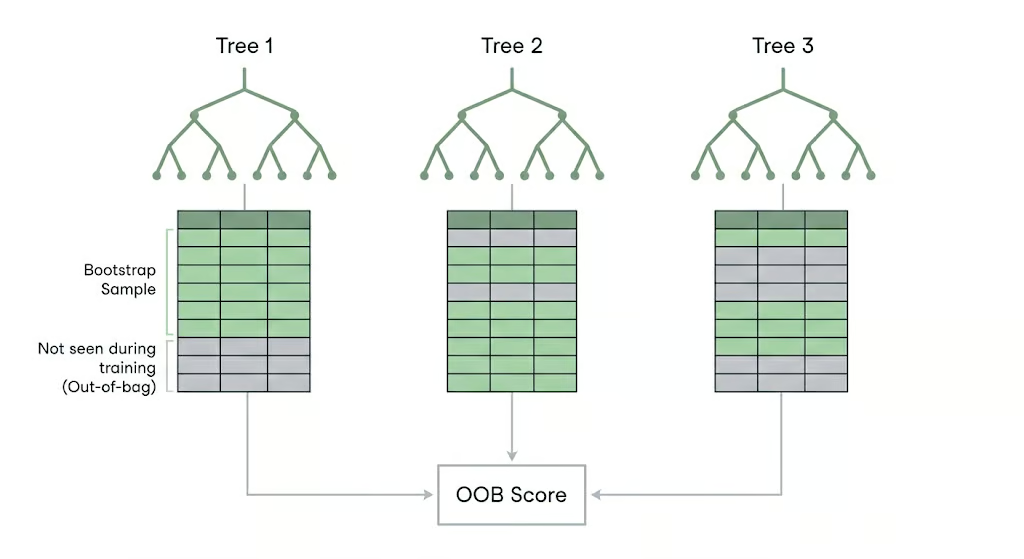
However, OOB evaluation is not always enough. For final model validation, especially in high-stakes scenarios or when data leakage is a concern, a strict hold-out test set is required. 

Prioritizing key hyperparameters for tuning

In Random Forest, max_features and n_estimators parameters typically drive the most noticeable changes in performance.

• max_features controls the maximum number of features considered at each split. Lower values increase randomness and reduce correlation between trees, which can improve generalization. Higher values make trees stronger but more similar, which potentially increases variance. 

• n_estimators controls the number of trees in the forest. Increasing it usually improves performance by stabilizing predictions, but it also increases computation time. Beyond a certain point, gains become marginal, so it is important to identify that plateau.

These parameters should be tuned using cross-validation to balance model complexity, training time, and predictive performance.

Feature Importance and Interpretability

Random Forest models are often treated as black boxes, but they provide multiple ways to understand how features influence predictions. Let’s see some important ones.

Impurity-based importance

Random Forest computes feature importance using Mean Decrease in Impurity (MDI). Each time a feature is used to split a node, the model measures how much that split reduces impurity, such as variance in regression tasks. These reductions are accumulated across all trees, giving a score that reflects how much a feature contributes to improving predictions.

While this method is fast and built into the model, it has known limitations. MDI tends to favor continuous features or categorical features with many unique values. These features create more potential split points, which can inflate their importance scores even if they are not truly more predictive.

Permutation importance

Permutation importance measures how performance changes when a feature’s values are randomly shuffled in a hold-out dataset. If shuffling a feature significantly degrades performance, that feature is important. If the impact is small, the feature likely has limited predictive value.

This approach reflects real model behavior, making it more trustworthy for analysis. 

However, correlated features introduce complexity. When two features carry similar information, shuffling one may not significantly impact performance because the other still provides the signal. As a result, importance can be split across correlated features, which requires careful interpretation.

SHAP value

SHAP values (Shapley Additive Explanations) explain how much each feature contributes to an individual prediction. It assigns each feature a value that represents how much it pushed the prediction above or below a baseline. 

This method is often used to explain model decisions and build trust. For a closer look, read our SHAP Values in Machine Learning tutorial.

Limitations and Common Failure Cases

Random Forest Regression is reliable across many scenarios, but it has clear limitations. Understanding these helps you decide when to use it and when to switch to a different approach.

Extrapolation limits and edge cases

Random Forest cannot extrapolate beyond the range of the training data. 

Each tree makes predictions based on splits observed during training, so the final output is always bounded by the minimum and maximum target values seen in the dataset. If the model has only seen targets between 10 and 100, it cannot predict 120, no matter how strong the input signal is. This becomes a problem in scenarios like growth forecasting or trend-driven systems. 

The model also struggles with extremely high-dimensional sparse data, such as text representations or one-hot encoded vectors with thousands of columns. In these cases, trees become inefficient and fail to capture meaningful splits. Practical workarounds include 

• Dimensionality reduction
• Feature selection
• Using models designed for sparse inputs, such as Ridge Regression

Interpretability trade-offs

A single tree provides a clear path from input to prediction, which makes it easy to explain. A forest, on the other hand, aggregates hundreds of trees, making individual decisions harder to trace.

In highly regulated environments, this trade-off matters. If explanations must be simple and directly traceable, a single decision tree or linear model may be more appropriate. If performance is the priority and explanations can be supported through methods like feature importance or SHAP, Random Forest remains a strong option.

Compute, memory, and latency constraints

Random Forest scales linearly with the number of trees and the size of the data. As datasets grow, training time and memory usage increase because each tree must be built and stored. Large forests can also slow down inference, since predictions require aggregating outputs from all trees.

In production systems with tight latency or cost constraints, this can become a bottleneck. Reducing the number of trees, limiting tree depth, or constraining the number of features considered at each split can help control resource usage. These adjustments trade some accuracy for faster training and prediction times.

Random Forest Regression vs. Alternatives: How To Choose

You might wonder if Random Forest Regression is the right algorithm for your use case, or which alternative you should consider.

Creating a model comparison framework

Use cases are different, but one approach always helps: Compare the performance of different models (like linear regression, support vector regression, gradient boosting, etc.) on the same dataset alongside the Random Forest Regressor. 

That means use the exact same train, validation, and test partitions for every model, then evaluate them under the same error criteria and business assumptions.

Random forest regression vs. linear regression and support vector regression

Random Forest and linear regression solve very different problems. Linear regression works best when the relationship between the inputs and target is mostly linear, and the coefficients need to be easy to explain. It is also the better choice when strict extrapolation matters, since it can extend beyond the observed target range. 

Random Forest, by contrast, is better at non-linear patterns, feature interactions, and irregular boundaries. That makes it a stronger modeling tool for complex real-world systems, but a weaker option for trend-heavy forecasting.

Support vector regression (SVR) sits in a different corner of the room. It can perform well on smaller datasets, but it is much more sensitive to feature scaling and usually needs more careful tuning. Random Forest does not depend on standardized inputs, which makes it easier to work with in typical tabular workflows. 

SVR can be a strong option when the dataset is compact and the feature space is limited, but it becomes harder to maintain as data volume, feature complexity, or operational pressure increases.

Random forest regression vs. gradient boosting and single decision trees

Random Forest builds trees independently and averages their outputs. Gradient boosting builds trees sequentially, where each new tree corrects the errors of the previous ones.

Gradient boosting methods, such as XGBoost, usually achieve higher accuracy ceilings, especially on structured tabular data. However, they require more tuning and are more sensitive to hyperparameters. Training can also be slower due to the sequential nature of boosting. Random Forest is easier to train, more stable out of the box, and less sensitive to configuration.

Compared to a single decision tree, Random Forest is far more stable and accurate. A single tree is easy to interpret because you can trace every decision path, but it is highly sensitive to small changes in the data. Random Forest reduces this instability by averaging across many trees, but it loses direct interpretability.

Model comparison summary

Final Thoughts

Random Forest Regression works best as a default model when the data is messy, relationships are non-linear, and you need a strong baseline without heavy preprocessing. It handles mixed feature types, captures interactions, and delivers stable performance with minimal setup.

The typical workflow follows a clear progression. Start with minimal preprocessing and focus on structuring the data correctly. Build a baseline using a default Random Forest model and evaluate it with consistent metrics. From there, tune key hyperparameters like the number of trees and feature sampling strategy to improve performance. 

Once the model stabilizes, move into deeper evaluation by analyzing residuals, slicing errors, and using SHAP to explain predictions where needed. 

As a next step, for a deep understanding and hands-on practice, check out this course on Machine Learning with Tree-Based Models in Python.