Heteroscedasticity: A Full Guide to Unequal Variance

If I could recommend learning one thing in depth to become a better data analyst or data scientist, it would be regression. And one key part of learning regression is understanding exactly what is heteroscedasticity.

In this article, we will look at the phenomenon of heteroscedasticity, learn why it matters, how to identify it, and steps to address it. I’ll be comprehensive but move quickly. So, if you’re a seasoned analyst or just getting started, I hope you will find something interesting and helpful here. For more information and to start the path to becoming an expert, take either our Intro to Regression in R course or our Intro to Regression in Python. I also have a tutorial on simple linear regression, if you need a quick recap.

What is Heteroscedasticity?

So what, exactly, is heteroscedasticity? Let’s get the technical definitions out of the way before we look at some examples. If you trip over the word like I do, you could say “unequal variance” and get the point across.

Heteroscedasticity refers to a situation in which the variability of a dependent variable is unequal across the range of values of an independent variable. Or, for a definition more anchored in model-building, we could say that heteroscedasticity happens when the spread or dispersion of residuals is not constant, as we sometimes see in a model like a regression model or a time series model.

In a way, I prefer this second definition because it reminds us that heteroscedasticity is actually a common aspect (though also a common problem) of statistical modeling. But just to be clear, while heteroscedasticity is most commonly discussed in the context of models like regression, it could be either a feature of the model specification or a property of the data itself.

Heteroscedasticity examples

Let’s look at some examples using R and pick an area - say, household finances. For starters, I will show the classic funnel or fan shape that I personally most think of when thinking of unequal variance.

This version of heteroscedasticity can occur, for example, in data with income vs. spending: Lower-income families often have consistent monthly spending focused on essentials like rent and food, resulting in low variability; higher-income families, on the other hand, may have more variability in spending because only some of the high-income households choose expensive discretionary purchases like vacations or luxury items, while others save. So, in this example, as income increases, the variability in monthly expenses also increases, hence the fan shape.

y_funnel <- x + rnorm(length(x), mean = 0, sd = x * 0.5)
y_inverse_funnel <- x + rnorm(length(x), mean = 0, sd = (1 / x) * 20)
y_cyclical <- x + rnorm(length(x), mean = 0, sd = 10 * abs(sin(x / 5)))

heteroscedasticity_data <- data.frame(x, y_funnel, y_inverse_funnel, y_cyclical)

library(ggplot2)

ggplot(heteroscedasticity_data, aes(x = x, y = y_funnel)) +
  geom_point(color = '#203147', alpha = 0.7) +
  geom_smooth(method = "lm", color = '#01ef63', se = FALSE) +
  labs(
    title = "Funnel Shape",
    x = "X Values",
    y = "Y Values"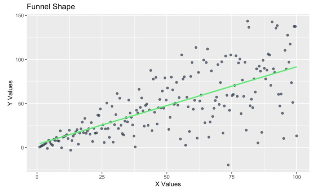
  )

Funnel-shape in the residuals. Image by Author

Let’s try another example, also in the realm of household finances. Imagine now that we are creating a regression model to show savings variability versus the age of household members.

We suspect this data will show heteroscedasticity because younger households might have high variability in savings due to irregular income, like gig work and internships, or unplanned expenses, like student loans or starting families. But as households age and stabilize financially, savings behavior becomes more consistent, creating an inverse funnel shape where variability decreases with age.

ggplot(heteroscedasticity_data, aes(x = x, y = y_inverse_funnel)) +
  geom_point(color = '#203147', alpha = 0.7) +
  geom_smooth(method = "lm", color = '#01ef63', se = FALSE) +
  labs(
    title = "Inverse Funnel Shape",
    x = "X Values",
    y = "Y Values"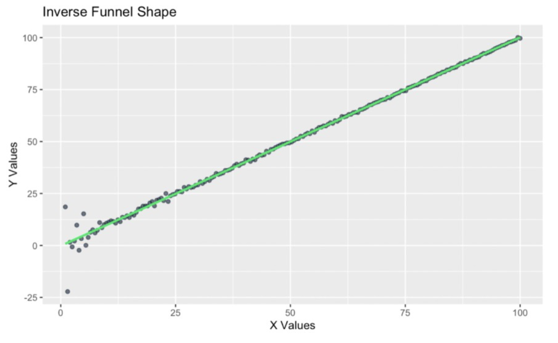
  )

Inverse funnel-shape in the residuals. Image by Author

Let’s look at a final example with household incomes. Here, we are looking at cyclical variance, specifically spending variance across seasons. You might recognize this kind of pattern if you have taken one of our forecasting courses, such as our very popular Forecasting in R.

We know that household spending often fluctuates cyclically throughout the year. For instance, variance might increase during holiday seasons because we buy gifts or travel to see family, and variance decreases in other months with fewer holidays, maybe March or September. The following graph shows heteroscedasticity but in a more complicated way, where it increases and decreases at different periods.

ggplot(heteroscedasticity_data, aes(x = x, y = y_cyclical)) +
  geom_point(color = '#203147', alpha = 0.7) +
  geom_smooth(method = "lm", color = '#01ef63', se = FALSE) +
  labs(
    title = "Cyclical Pattern",
    x = "X Values",
    y = "Y Values"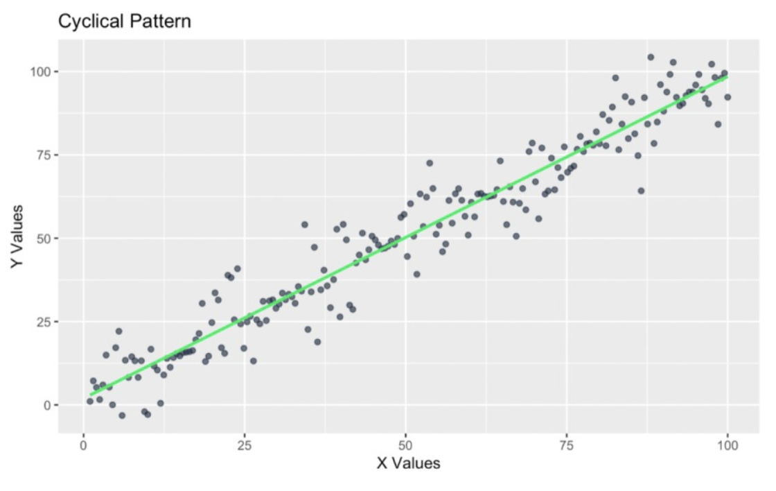
  )

Cyclical pattern in the residuals. Image by Author

So, as you can see, heteroscedasticity can take several forms. Let's now look at why all this matters.

Importance in statistical modeling

I would venture to say that, generally speaking, you can’t do regressions correctly without understanding something about heteroscedasticity since heteroscedasticity is so common and can have such a big effect distorting our results.

It’s probably for this reason that homoscedasticity - the opposite of heteroscedasticity - is actually one of the main regression model assumptions, along with linearity, independence of errors, normality of residuals, and the absence of multicollinearity.

These regression assumptions matter because they help make sure that our model’s predictions and inferences are meaningful. When these assumptions are violated, the reliability of our estimates, including our standard errors and confidence intervals, can be degraded, and our hypothesis tests are less valid.

Causes of Heteroscedasticity

Heteroscedasticity doesn’t appear out of nowhere. Its roots often lie in how data is collected or transformed. Let’s look at both data transformation issues and data collection issues.

Data transformation issues

Sometimes, the very steps we take to prepare our data can introduce heteroscedasticity. I'm thinking about how improper scaling or nonlinear transformations can create unintended variability.

To think about this, let’s imagine we are studying the relationship between the size of an apartment and its monthly rent. Normally, we might expect a linear relationship between size and rent because larger apartments cost more, and the variance in rent might not necessarily increase with size because the relationship (might be) proportional. Here is what that might look like:

set.seed(1024)

size <- runif(1000, 500, 2000) # Random sizes between 500 and 2000 sq ft
rent <- 20 * size + rnorm(100, mean = 0, sd = 5000) # Linear relation with added noise

unequal_variance_df <- data.frame(size = size, rent = rent)

ggplot(unequal_variance_df, aes(x = size, y = rent)) +
	geom_point(color = '#203147', alpha = 0.7) +
	geom_smooth(method = "lm", color = '#01ef63', se = FALSE) +
	labs(title = "Size vs. Rent",
	    x = "Size (sq ft)",
	    y = "Rent")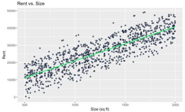

No heteroscedasticity. Image by Author

What happens when we scale by size?

If we scale rent by size to compute "rent per square foot," we create a new metric. If we then try to predict rent per square foot by rent, we might see that this transformation creates or exaggerates heteroscedasticity. To be clear, in general, I acknowledge this is not a good idea - to divide the independent variable by the dependent variable - because we are creating a situation where y is already influenced by x and we are therefore creating a spurious correlation. So, I recognize that this creates conceptual and statistical challenges. But (bear with me) I'm using this as an example to try to illustrate the point:

unequal_variance_df$rent_per_sqft <- unequal_variance_df$rent / unequal_variance_df$size

ggplot(unequal_variance_df, aes(x = size, y = rent_per_sqft)) +
	geom_point(color = '#203147', alpha = 0.7) +
	geom_smooth(method = "lm", color = '#01ef63', se = FALSE) +
	labs(title = "Size vs. Rent per Square Foot",
	     x = "Size (sq ft)",
	     y = "Rent per Sq Ft")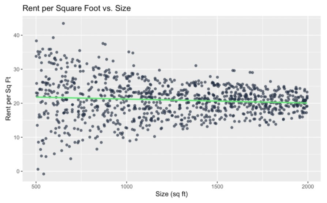

Heteroscedasticity induced as a result of functional dependency. Image by Author

We can see this graph has a funnel shape where the variability in rent per square foot decreases as the size increases. So, we've created heteroscedasticity out of nothing. For another example, we can square both variables:

unequal_variance_df$size_squared <- unequal_variance_df$size^2

ggplot(unequal_variance_df, aes(x = size ^ 2, y = rent ^ 2)) +
	geom_point(color = '#203147', alpha = 0.7) +
	geom_smooth(method = "lm", color = '#01ef63', se = FALSE) +
	labs(title = "Size Squared vs. Rent Squared",
	     x = "Size Squared",
	     y = "Rent Squared")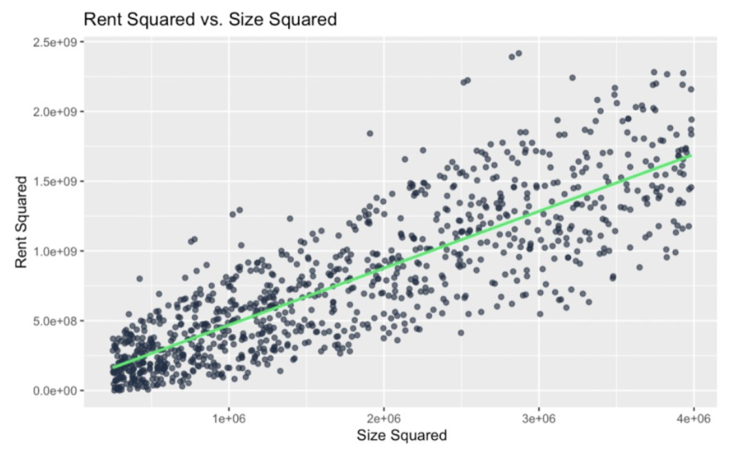

Heteroscedasticity induced as a result of squaring. Image by Author

Again, we've created heteroscedasticity where none existed before because we insisted on squaring both the x and y. In some contexts, this would be fine, but here I suspected that squaring both variables would create heteroscedasticity because I thought the transformation would amplify differences in variance as the values of the variables increased.

This second example is also a bit contrived because we shouldn't make this model. We wouldn't make this model because it would be hard to interpret for no reason. But, in a real-world modeling workflow, transformations that inadvertently create heteroscedasticity can be more subtle. You might miss it if the process involves multiple steps.

More exactly, in this case, heteroscedasticity has resulted from feature engineering with ratios. Ratios like "rent per square foot" are indeed common in feature engineering. However, these variables can introduce heteroscedasticity if the denominator, in particular, varies significantly across observations. Logarithmic or exponential transformations are also frequently used to stabilize variance or linearize relationships. However, applying them inconsistently can backfire. Suppose you have a model where you log-transform income but fail to adjust related features like expenditures. This kind of mismatch is a common source of heteroscedasticity, so make sure everything aligns so you don't induce false dynamics.

Variability in data collection

Heteroscedasticity can also stem from inconsistent data collection practices. For example, switching up the measurement tool part way through a study could introduce heteroscedasticity. Having different size groups and, therefore, different sample sizes in a study can also create heteroscedasticity. Sticking with one approach matters.

Detecting Heteroscedasticity

Detecting heteroscedasticity is the first step toward addressing it, and fortunately, there are both visual and statistical tools to help.

Visual inspection techniques

Scatter plots can reveal patterns in your data that help uncover heteroscedasticity. I like the fitted values vs. residuals plot for this. As a note, a histogram of residuals or a residual q-q plot is not enough to detect heteroscedasticity because these two plots are really best used for testing normality.

y_funnel <- x + rnorm(length(x), mean = 0, sd = x * 0.5)

heteroscedasticity_data <- data.frame(x, y_funnel)

unequal_variance_model <- lm(y_funnel ~ x, heteroscedasticity_data)

fitted_values_vs_residuals <- ggplot(data = unequal_variance_model, aes(x = .fitted, y = .resid)) +
    geom_point(color = '#203147') +
    geom_hline(yintercept = 0, linetype = "dashed", color = '#01ef63', size = 1) +
    xlab("fitted values") +
    ylab("residuals") +
    labs(title = "Heteroscedasticity Data") +
    labs(subtitle = "Fitted Values vs Residuals")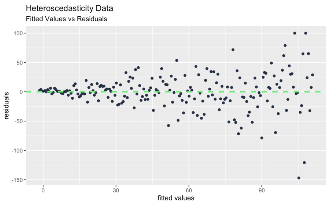

Fitted values vs. residuals diagnostic plot. Image by Author

Statistical tests

Statistical tests like the Breusch-Pagan test offer a more quantitative approach. The Breusch-Pagan works by looking at whether the squared residuals from the model are related to the predictors. To conduct the test, we fit our model and use the bptest() function from the lmtest library. Do know the test does assume normal residuals.

library(lmtest)

model <- lm(rent ~ size, data = unequal_variance_df)

bp_test <- bptest(model)

print(bp_test)

Addressing Heteroscedasticity

Once you’ve identified heteroscedasticity, the next step is to tackle it using proven techniques.

Data transformation methods

Simple transformations, like applying logarithms, can often reduce or eliminate heteroscedasticity. Earlier, we took a model without unequal variance, applied transformations and created problems, but more naturally the opposite workflow happens: We use transformations like logarithms, square roots, or reciprocals to compress larger values while expanding smaller ones. For example, if rent instead grew exponentially with size, taking the log of rent would flatten the exponential growth and make the relationship linear with (maybe) equal variance.

Also, I want to point out that when we are prepping data, we often think about fixing skewness. For example, if we have right-skewed data, we might use a square root transformation to make the data Gaussian. But what we might not appreciate as much is that in skewed data, larger values also tend to have greater variability, which is a violation of the assumptions of homoscedasticity, also.

Robust regression techniques

When transformations aren’t enough, robust regression methods like weighted least squares (WLS) can help. Weighted least squares is especially interesting here because it is designed to handle data issues such as heteroscedasticity and outliers. Specifically, WLS assigns weights to observations based on their variance, thus reducing the influence of data points with higher variability, and thus giving us more stable estimates. As a note, with WLS, we would assume the weights are well-known or well-estimated.

Implications of Ignoring Heteroscedasticity

Ignoring heteroscedasticity might seem harmless, but it can lead to problems.

Impact on model accuracy

Heteroscedasticity can distort how a model interprets the importance of features. For example, in a spending model, features like income might seem more important if they are linked to groups with high variability, such as high-income households with discretionary purchases. This misrepresentation can lead us to overemphasize less reliable predictors while underestimating more consistent ones, affecting the model's usefulness.

Consequences for hypothesis testing

Heteroscedasticity can invalidate the use of common statistical tests like t-tests or F-tests if you are assuming equal variance and this assumption is not met. Unequal variance is also problematic in time-series data, where patterns of variability evolve over time, leading to confusion when analyzing seasonal trends. Heteroscedasticity-consistent standard errors (HCSE) could be used to help enable more reliable statistical inference.

Related Ideas

In this article, we have studied the situation where the variance of the residuals is not constant across levels of an independent variable in a model. Here, I want to talk briefly about a related idea, which is group-level variance heterogeneity, referring to variability across predefined groups, which is less a statistical issue tied to model assumptions and more of a descriptive observation of the data.

I'll show with a final example. Here, I'll be using a simulation of survey data. I'm considering a scenario where income data is collected using two different methods: surveys and admin records. These methods might have different levels of precision (Aren't surveys notorious?). We can see that the amount of variation within each group is not consistent, which could be a problem with something like ANOVA.

set.seed(1024)

income_admin <- rnorm(500, mean = 50000, sd = 2000) 
spending_admin <- income_admin * 0.3 + rnorm(500, mean = 0, sd = 1000)
income_survey <- rnorm(500, mean = 50000, sd = 8000) # Same mean, higher SD
spending_survey <- income_survey * 0.3 + rnorm(500, mean = 0, sd = 5000)
income <- c(income_admin, income_survey)
spending <- c(spending_admin, spending_survey)
method <- rep(c("Administrative Records", "Survey"), each = 500)

survey_and_admin_data <- data.frame(income = income, spending = spending, method = method) # Plot the data

custom_colors <- c("Administrative Records" ='#01ef63', "Survey" = '#203147')

ggplot(survey_and_admin_data, aes(x = income, y = spending, color = method)) +
  geom_point(alpha = 0.7) +
  labs( title = "Variability in Data Collection", x = "Income", y = "Spending")+
  scale_color_manual(values = custom_colors)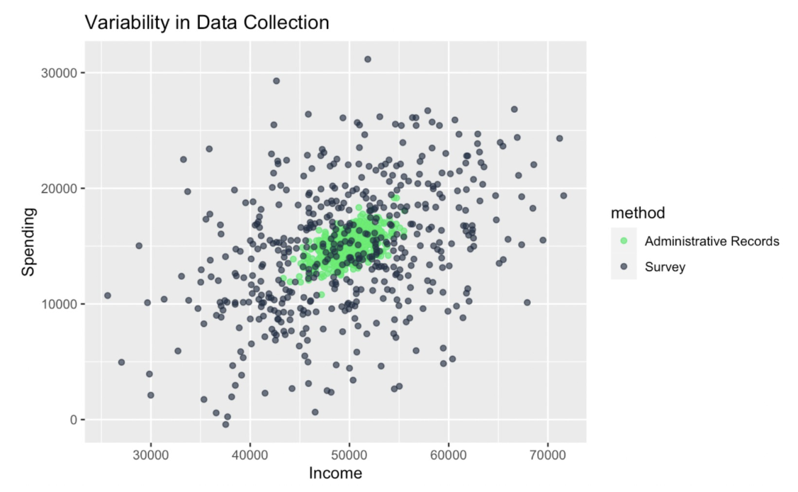

Group-level variance heterogeneity. Image by Author

Conclusion

Addressing heteroscedasticity isn’t just about improving your regression model. It’s about making sure your work stands up to scrutiny. To keep learning and become an expert, take our Statistical Inference in R track and Foundations of Inference in R course. I also think our Statistician in R track is another great option for both learning and career development.