Support Vector Regression (SVR): How It Works and When to Use It

Standard regression methods minimize total error across all data points. That means every residual, no matter how small, pulls the model in some direction. As the result, you end up with a model that's sensitive to noise and outliers.

A support vector regression model, on the other hand, fits a function within a tolerance margin and ignores errors that fall inside it. That margin changes the idea of optimization. Instead of trying to optimize every data point, SVR focuses on the overall structure of the data, which makes it, as I hope to show you, robust on real-world data.

If you need a primer before we get started, read our Linear Regression in Python article for an introduction to predictive modeling.

What Is Support Vector Regression?

Support Vector Regression is a regression method built on the same foundation as Support Vector Machines (SVM), which is a class of models originally designed for classification tasks like spam detection or image recognition.

The key idea is easy to understand - instead of trying to minimize every prediction error, SVR fits a function while allowing a margin of tolerance around it. Errors that fall within that margin don't count. The model focuses on getting the overall fit right, not on correcting every small deviation.

That’s what sets SVR apart from most other regression models.

Standard regression methods treat every residual as a signal. SVR treats most of them as noise. As a result, you end up with a model that's less concerned with being exactly right on every point and more concerned with getting the underlying structure of the data right.

The Core Idea Behind SVR

At the center of SVR is something called the epsilon tube - a margin of tolerance that wraps around the fitted function on both sides.

Any data point that falls inside the tube is considered close enough. SVR ignores those points when fitting the model. Only the points outside the tube matter, as those are the ones that actually shape the decision boundary.

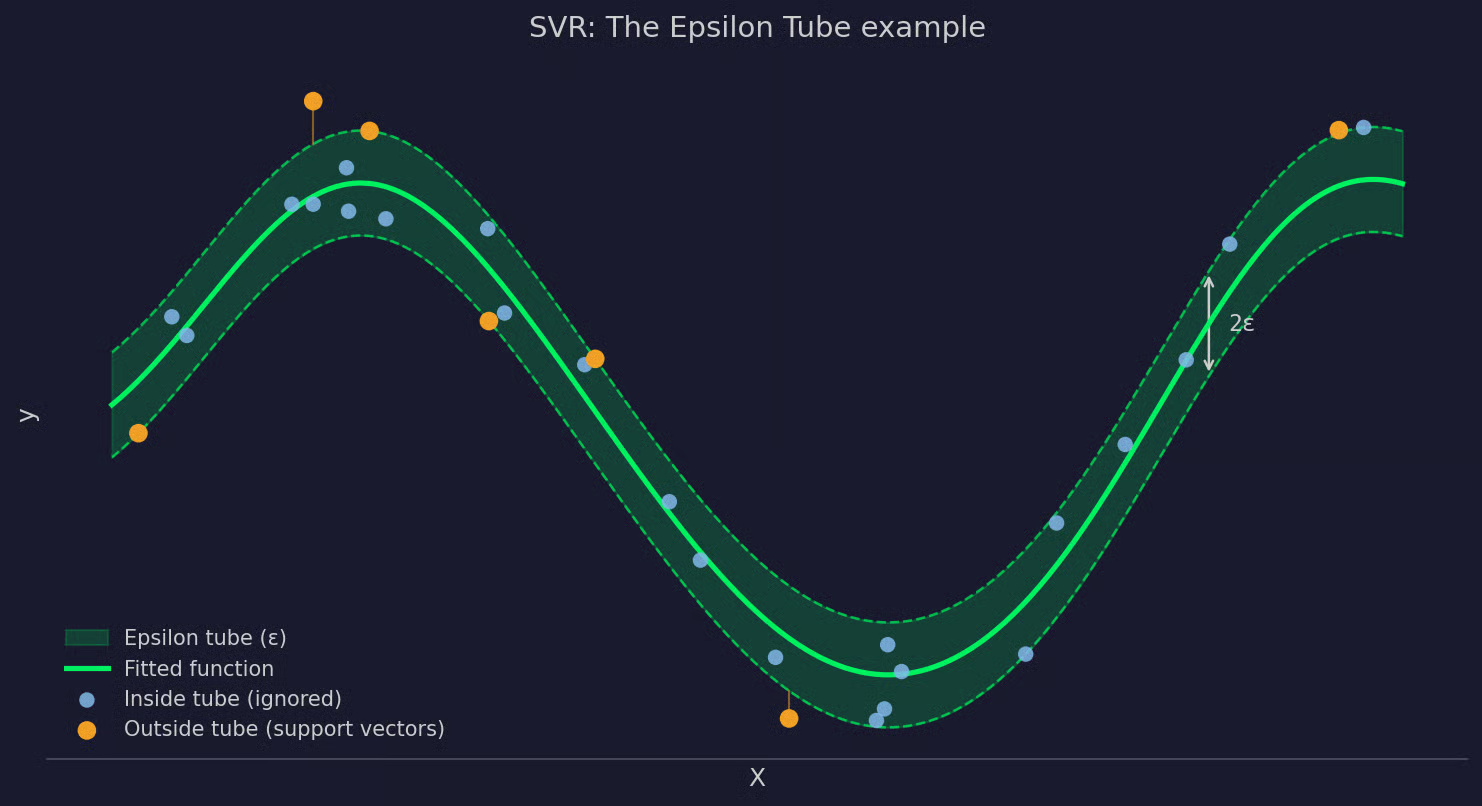
The Epsilon tube example

Here's how you can interpret it:

• Points inside the tube contribute zero error, regardless of how far they are from the function
• Points outside the tube contribute an error proportional to how far they sit beyond the margin
• The model is defined by those outside points, not by the majority of the data

This is what separates SVR from standard regression. In linear regression, every data point pulls on the model - including the noisy ones. In SVR, most points are irrelevant. The result is a fit made by overall good structure.

How SVR Is Optimized

SVR has two competing goals it tries to satisfy at once.

The first is to keep the model as flat as possible. A flatter function is simpler, and simpler models tend to generalize better to new data. The second is to minimize errors on points outside the epsilon tube - the ones SVR can't ignore.

These two goals pull in opposite directions, and that's where the regularization parameter C comes in. It controls how much weight SVR puts on errors outside the tube relative to model simplicity:

• A high C value tells the model to take outside errors seriously, which can produce a more complex, tightly fitted function
• A low C value lets the model stay simple and accept more violations outside the margin

You're always trading off model simplicity against error tolerance. The right value of C depends on your data and how much noise you expect. Getting it wrong in either direction will decrease your model's performance on new data.

It’s an optimization problem that can be solved iteratively, so it’s nothing to worry about.

Support Vectors in SVR

With SVR, only the data points that fall outside the epsilon tube actually matter.

These are the support vectors - the data points that sit beyond the margin and shape the fitted function. Everything inside the tube is ignored during training. The model never "sees" those points in any meaningful way.

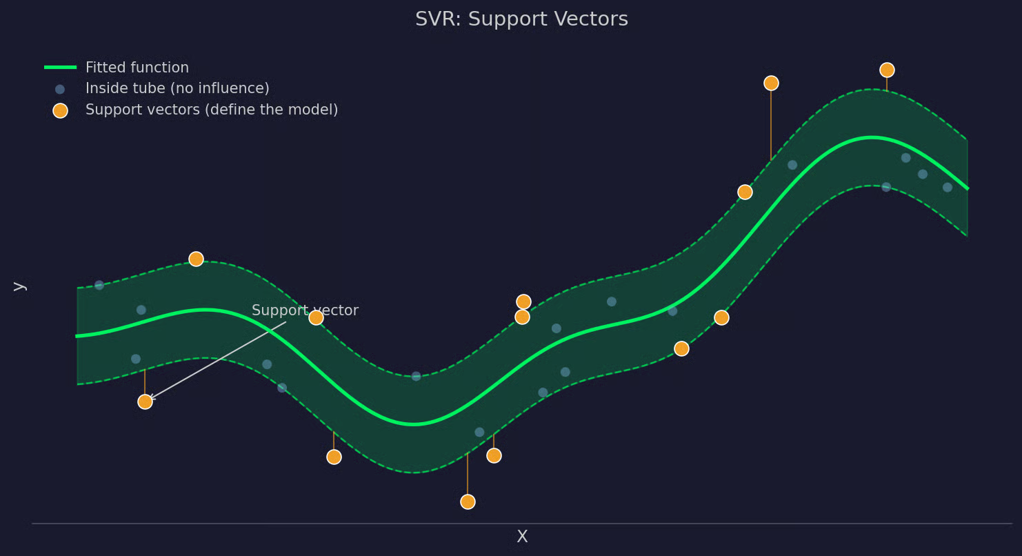
Support vectors

The useful side effect of this is sparsity. In practice, only a small subset of your training data ends up as support vectors. The rest contributes nothing to the final model, which makes SVR memory-efficient and fast to evaluate once it's trained, since predictions depend only on those few influential points.

Handling Nonlinear Data with SVR

SVR isn't limited to fitting straight lines. It can handle nonlinear relationships through a technique called the kernel trick.

So, instead of fitting a function in the original input space, SVR maps the data into a higher-dimensional space where a linear fit becomes possible. That linear fit in the higher-dimensional space translates back to a nonlinear curve in your original data.

The two most common kernels you'll use are:

• RBF (Radial Basis Function): The default choice for most problems. It handles smooth, curved relationships well and works across a wide range of datasets
• Polynomial: Useful when you have reason to believe the relationship follows a polynomial pattern of a specific degree

How you choose the kernel depends on your data. RBF is a good starting point when you're not sure.

SVR vs Linear Regression

The difference comes down to what each model is trying to do.

Linear regression minimizes total error across every data point. Every residual counts, no matter how small it is. If you pull the model off course with a noisy point, the whole fit shifts to compensate.

SVR ignores errors within the epsilon tube. It only reacts to points that fall outside the margin - and even then, C controls how strongly. The model is optimizing for structure, not for accuracy on every individual point.

That difference makes SVR more robust to outliers. A single noisy point won't run the fit the way it can in linear regression, because SVR was never trying to chase it in the first place.

Here are all the differences:

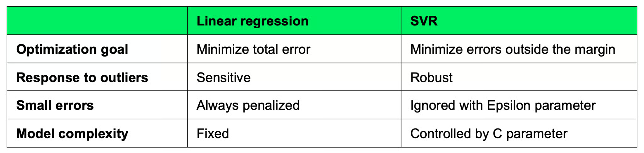
Linear regression compared to SVR

Key Parameters in SVR

SVR has three parameters you need to understand before you start optimizing the model.

Epsilon (ε)

Epsilon defines the width of the tolerance margin around the fitted function. A larger ε means a wider tube - more points are ignored and the model gets simpler. A smaller ε tightens the tube and forces the model to fit more closely to the data.

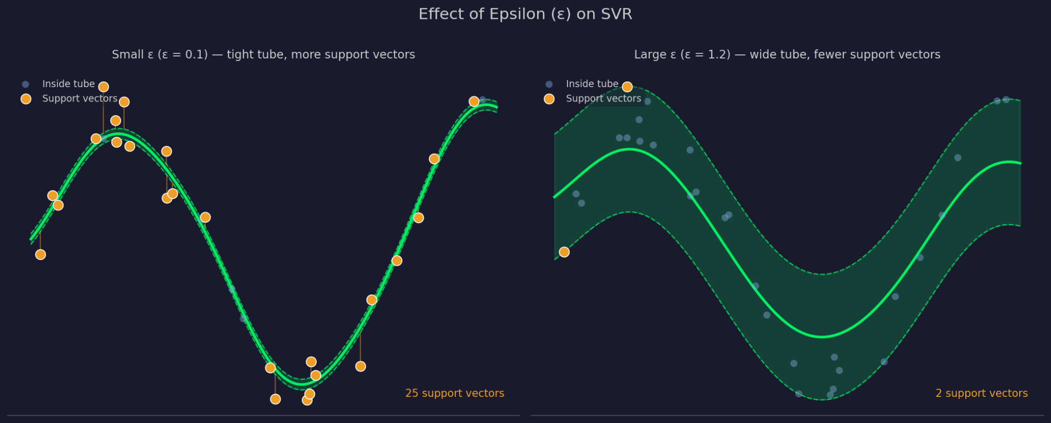
Small versus large Epsilon

C (regularization)

C controls how much SVR penalizes errors on points outside the tube. High C means the model takes those errors seriously and fits more tightly. Low C means the model accepts more violations in exchange for a simpler, flatter function. C and ε work together, as changing one affects how the other behaves in practice.

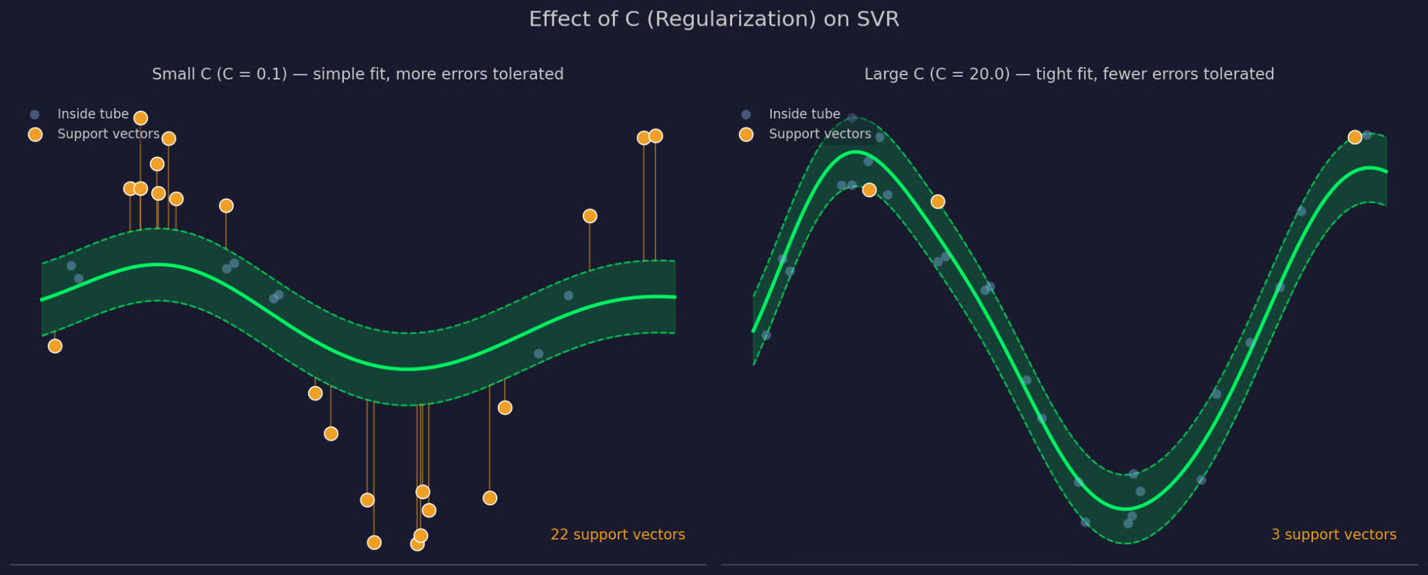
Small versus large C

Kernel

The kernel determines how SVR handles nonlinear patterns. RBF is the most common choice and works well as a default. Polynomial kernels are useful for specific curve shapes. Linear kernels reduce SVR to a margin-based linear regression, which can be useful when your data is already well-behaved.

Support Vector Regression in Practice

Getting SVR to work well is about going through a couple of steps and prerequisites. Let me show you what these are.

Here's the typical workflow:

1. Scale your data: SVR is sensitive to feature scale. If your features are on different scales, the model won't behave as expected. Use StandardScaler on both X and y before fitting

2. Choose a kernel: RBF is the right default for most problems. Switch to a polynomial if you have a specific reason to believe the relationship follows that shape

3. Tune your parameters: Set C, epsilon, and gamma before fitting. Grid search or cross-validation are the standard approaches here

4. Fit the model: Call .fit() on the scaled training data. Once it's trained, inverse-transform your predictions back to the original scale

Here's a complete example using scikit-learn:

import numpy as np
from sklearn.svm import SVR
from sklearn.preprocessing import StandardScaler
from sklearn.model_selection import train_test_split
from sklearn.metrics import mean_squared_error

# Generate sample data
np.random.seed(42)
X = np.sort(np.random.uniform(0, 10, 30))
y = 2.5 * np.sin(X * 0.8) + np.random.normal(0, 0.4, 30)

# Split
X_train, X_test, y_train, y_test = train_test_split(
    X, y, test_size=0.2, random_state=42
)

# Scale features and target
scaler_X = StandardScaler()
scaler_y = StandardScaler()

X_train_scaled = scaler_X.fit_transform(X_train.reshape(-1, 1))
X_test_scaled = scaler_X.transform(X_test.reshape(-1, 1))
y_train_scaled = scaler_y.fit_transform(y_train.reshape(-1, 1)).ravel()

# Fit SVR
svr = SVR(kernel="rbf", C=2.0, epsilon=0.5, gamma=0.3)
svr.fit(X_train_scaled, y_train_scaled)

# Predict and inverse-transform
y_pred_scaled = svr.predict(X_test_scaled)
y_pred = scaler_y.inverse_transform(y_pred_scaled.reshape(-1, 1)).ravel()

rmse = np.sqrt(mean_squared_error(y_test, y_pred))
print(f"Test RMSE: {rmse:.3f}")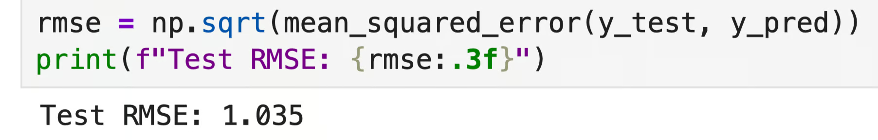

RMSE on the test set

A couple of things to notice in this code. First, StandardScaler is applied to both X and y separately. Scaling only the features is a common mistake that leads to poor results with SVR. Second, predictions are inverse-transformed at the end to bring them back to the original scale before evaluation.

The two plots below show what the fitted model looks like. The first shows the SVR curve with the epsilon tube over the training and test data:

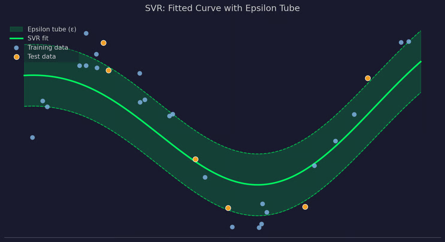
Epsilon tube over the training and test data

The second compares predicted versus actual values on the test set:

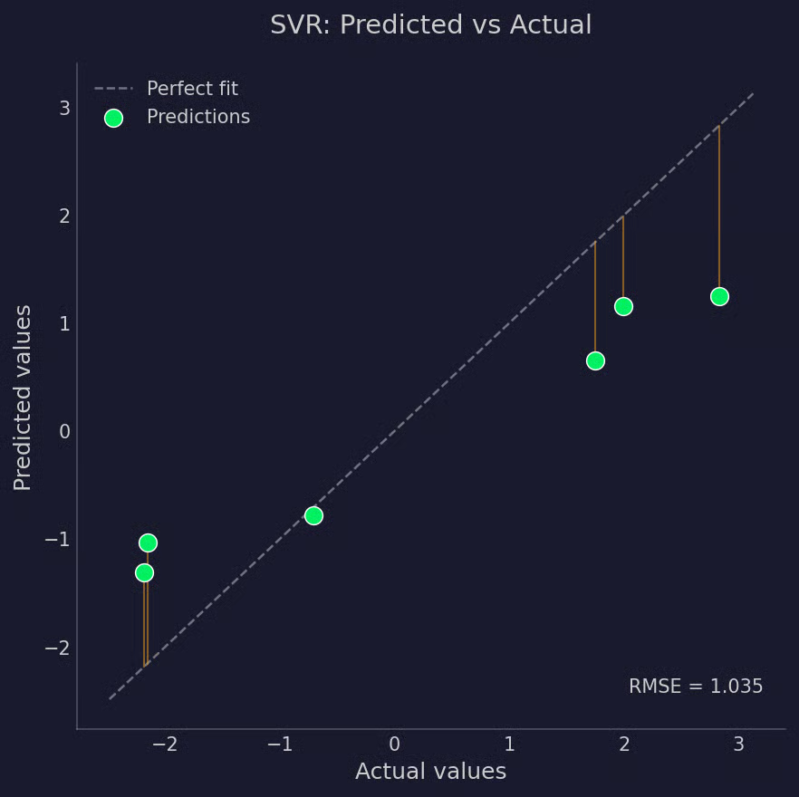
Predicted versus actual values

Points close to the diagonal mean the model is predicting well.

Advantages and Limitations of SVR

SVR has a specific set of strengths that make it the right tool in the right situation. Similarly, it has weaknesses that make it the wrong one in others.

Advantages

• Robust to noise: The epsilon tube means small errors don't influence the model at all. Noisy data that would pull a model like linear regression off course gets ignored
• Handles nonlinear relationships: With the right kernel, SVR fits curves that standard regression can't without manual feature engineering
• Flexible: You control the margin width, the penalty for errors, and the kernel, which means you can adapt the model to a wide range of data shapes and noise levels

Limitations

• Slow on large datasets: SVR doesn't scale well. Training time grows as the number of samples increases, which makes it impractical for datasets with hundreds of thousands of rows or more.
• Sensitive to parameter tuning: C, epsilon, and gamma all interact with each other. A bad combination will decrease performance, and finding a good one takes time and compute, especially as SVR doesn’t scale well
• Less interpretable: There's no simple coefficient to inspect. Understanding why SVR made a particular prediction isn't easy, so if explainability is a must-have in your line of business, this isn’t the model for you

When to Use SVR

SVR works best in a specific set of conditions. You should use SVR when:

• Your dataset is moderate in size - a few hundred to a few thousand samples is the sweet spot
• The relationship between features and target is nonlinear and you don't want to engineer features manually
• Your data has noise or outliers and you need a model that won't be affected by them

You should avoid SVR when:

• Your dataset is very large - training will be slow and may not finish in a reasonable time
• Speed matters - both training and hyperparameter search are expensive compared to alternatives like gradient boosting or linear regression

If your dataset is large and noisy, gradient boosting methods are worth looking at first. SVR is great when you have clean, moderate-sized data with structure that simpler models can't fit well.

Common Mistakes with SVR

Most issues with SVR come down to the same set of errors - so treat this as a cheat sheet of what not to do.

• Not scaling your features. SVR is a distance-based algorithm, which means unscaled features will dominate the model. Always apply StandardScaler to both X and y before fitting.

• Misunderstanding epsilon. Epsilon is by far the most important parameter. Too large and your model underfits as it ignores too much. Too small and it behaves like standard regression, chasing every data point. Always do a grid search to see what performs best on your test set.

• Skipping parameter tuning. Running SVR with default parameters and expecting good results rarely works - just like with most machine learning models. C, epsilon, and gamma need to be tuned together. Use grid search with cross-validation.

• Using SVR on very large datasets. If you have more than a few thousand samples, SVR will be slow. It just doesn’t scale like other algorithms do. Switch to a model that works with large datasets better, like gradient boosting or a neural network.

It’s also important to note that getting these four things right won't guarantee a great model, but getting any of them wrong will almost certainly guarantee a bad one.

Conclusion

To conclude, remember that SVR solves a different problem than standard regression. Instead of minimizing every error, it fits a function within a margin and ignores the noise that falls inside it - which is exactly what makes it useful when your data isn't clean or perfectly linear.

It isn’t well-known for its speed or simplicity. But it’s robust. If your data has nonlinear relationships and outliers you don’t want to model, SVR will give you a way to focus on structure rather than chasing every data point.

Just remember to scale your features, tune your parameters, pick the right kernel, and stay conservative with the amount of data. If you do these right, SVR will give you a robust model that isn’t likely to fail in production.

SVR is just one tool every data scientist has to know. Enroll in our Machine Learning Engineer track to learn the others and get job-ready in 2026.