Measures of Central Tendency: A Comprehensive Overview

Central tendency is one of the most significant concepts in statistics, describing the typical value around which data tend to cluster. It provides a single, representative number that summarizes an entire dataset, making large quantities of information digestible and comparable.

Historically, the idea of a “central value” has evolved over centuries. Ancient scholars like the Greeks considered simple averages, while mathematicians in the 17th and 18th centuries formalized mean, median, and mode as statistical tools. The 20th century brought further sophistication, introducing specialized measures for working with skewed or outlier-prone data. Today, central tendency remains crucial in a wide spectrum of fields, from social sciences and economics to engineering and machine learning.

Fundamental Concepts of Central Tendency

Before I go into the variants, let's review some of the terminology. For a closer and more comprehensive look at this and more, enroll in our Introduction to Statistics course.

Definition and purpose

Central tendency refers to the statistical measure that identifies a central point within a dataset. It functions as a summary statistic, indicating where most values in the distribution tend to cluster. By offering a single, representative value, it simplifies the complex variability inherent in raw data.

A key purpose of central tendency is to enable comparisons between datasets. For instance, using central measures, we can compare average incomes across cities and reveal socioeconomic patterns quickly. Importantly, central tendency differs from measures of dispersion, which describe how data spread around the center. While the mean or median shows where the data center lies, measures like variance and standard deviation reveal how tightly or loosely data is distributed around that center.

Role in descriptive statistics

In descriptive statistics, central tendency is used to effectively summarize large datasets. Whether analyzing exam scores, production times, or customer ratings, knowing the typical value is invaluable for interpreting trends.

Central tendency interacts closely with variability measures. For example, two datasets might have the same mean but differ dramatically in spread, influencing how reliable that mean truly is as a summary statistic. 

In real-world scenarios, central tendency helps policymakers, business leaders, and researchers make decisions based on representative values. A retailer may analyze average sales to develop inventory strategies, while a healthcare researcher might examine median survival times to assess treatment efficacy.

Types of data and central tendency

Choosing an appropriate measure of central tendency depends heavily on the data type. Data fall into four broad categories:

• Nominal data represent categories without inherent order (e.g., blood types, colors).
• Ordinal data indicate ranked order but without consistent intervals (e.g., survey ratings like poor, fair, good).
• Interval data have ordered values with equal intervals but no true zero (e.g., Celsius temperatures).
• Ratio data feature equal intervals and an absolute zero (e.g., weight, height, income).

Here are the most suitable measures of central tendency for each type of data:

• For nominal data, the mode is appropriate because averaging categories like “red,” “blue,” and “green” is meaningless.
• For ordinal data, the median is often the best choice, respecting rank without assuming equal differences between ranks.
• For interval and ratio data, the mean, median, or mode might all be good, depending on the data’s distribution and presence of outliers.

For example, median household income is frequently reported because income data are skewed by extreme high earners, while mean height is reasonable for normally distributed human heights.

Primary Measures of Central Tendency

There are three primary measures of central tendency: the arithmetic mean, median, and mode. Let’s consider each of them, paying special attention to their strengths and limitations.

Arithmetic mean

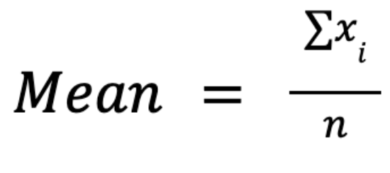
The arithmetic mean, often simply called the average or the mean, is calculated by summing all values in a dataset and dividing by the number of observations:

The main advantage of this measure is in its mathematical properties: it’s algebraically manipulable, allowing for elegant formulations in inferential statistics, hypothesis testing, and regression analysis. For example, it integrates seamlessly into variance and standard deviation calculations.

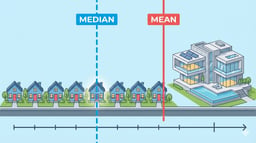
However, the mean is highly sensitive to outliers: a few extreme values can skew it significantly, making it unrepresentative for skewed distributions. For instance, in income data, several billionaires can raise the mean far above what most people earn.

Talking about the mean, it’s crucial to distinguish between the population mean (μ) and the sample mean (x̄). The first of them describes the entire population, while the latter estimates it from a subset. To draw conclusions about the whole population from a sample of data, we use a process called statistical inference.

Scenarios where the mean should not be used include heavily skewed distributions, data with significant outliers, or ordinal data, where averaging ranks has no practical meaning.

Median

The median represents the middle value of an ordered dataset. For an odd number of values, it’s the single center value. For an even-numbered dataset, it’s the average of the two middle values.

To calculate the median, we need:

1. To order the data from smallest to largest.
2. To identify the middle value.

The key strength of the median is its robustness to outliers: extreme values at either end of the distribution have no influence on its value, making it ideal for skewed data such as income or property prices.

However, the median is mathematically less manageable than the mean. It’s less useful in complex statistical formulas or modeling and does not integrate easily into algebraic manipulations.

Mode

The mode is the value occurring most frequently in a dataset. Unlike mean and median, it can be used also with nominal data, making it applicable across different data types.

The mode helps identify high-frequency categories, such as the most popular product color or the most common customer complaint. However, it has some limitations:

• In uniform distributions, there may be no mode.
• In multimodal distributions, there can be several modes, which complicates interpretation.
• For numerical data, the mode can be less informative, up to being meaningless if all values are unique.

A frequency distribution table often helps determine the mode. For instance, in the below frequency distribution table of apple colors, “green” is the mode:

Comparative Analysis of Primary Measures

Understanding how mean, median, and mode differ in performance and suitability is critical in statistics. Let's compare them:

Sensitivity to outliers and skewness

Among the three measures, the mean is the most sensitive to outliers: a single extreme value can distort the mean significantly. The median, by contrast, remains stable unless enough extreme values accumulate to shift the middle point. The mode is completely insensitive to outliers because it depends purely on frequency.

Skewness also affects these measures. In right-skewed distributions (e.g., income data), the mean typically is higher than the median, which in turn is higher than the mode.(By mode here, I mean the mode in a continuous distribution, where mode is the peak of the probability density curve, assuming that one exists.)

Conversely, in left-skewed distributions (e.g., test scores where most students score high), the mean falls below the median and mode:

Symmetrical distributions, like the normal distribution, ideally show equality among all three measures:

In practice, however, small deviations may occur in symmetrical distributions due to sampling variability.

Relationships among mean, median, and mode

In the previous section, we’ve already seen the overall relationships among mean, median, and mode in normal and skewed distributions. In general, the relationships among the three measures serve as a diagnostic tool for skewness. In empirical studies, statisticians often apply Pearson’s second skewness coefficient:

For instance, in salary distributions, a significant gap between the mean and median signals income inequality. Similarly, in housing markets, the median home price often better reflects typical costs than the mean, which can be skewed by a few extremely expensive properties.

Applicability by data type

Different central tendency measures fit different data types. The table below summarizes optimal use cases and limitations for each measure.

As we see, it’s important to align the statistical measure with the nature of the data.

Specialized Measures of Central Tendency

Apart from the primary measures of central tendency, there are specialized alternatives that address specific data challenges like skewness, outliers, and data scaling.

Trimmed and winsorized means

A trimmed mean excludes a fixed percentage of extreme values from both ends of the dataset before calculating the average. For example, a 10% trimmed mean removes the lowest 10% and highest 10% of values.

A winsorized mean doesn’t eliminate extreme values but replaces them with the nearest remaining values. This measure is useful in fields like finance, manufacturing, and survey analysis where data can include rare but influential extremes.

Both techniques reduce the influence of outliers, achieving a balance between robustness and data retention by combining the mean’s sensitivity with the median’s resilience.

Geometric and harmonic means

The geometric mean multiplies all data points and takes the nth root (where n is the number of data points). It’s particularly useful in multiplicative processes, such as growth rates, investment returns, and biological measurements. The formula for calculating the geometric means is as follows:

For example, average growth over multiple years is better summarized with a geometric mean than an arithmetic mean.

The harmonic mean is calculated as:

It’s valuable when averaging rates, like speed or financial ratios. For example, in calculating average speed over different distances, the harmonic mean gives the correct overall rate.

Weighted and trimean measures

A weighted mean assigns varying importance to data points. For example, a student’s final grade may combine exam scores and coursework with different weights. This measure adjusts for biases and ensures that more significant observations have more influence.

The trimean combines the median and quartiles:

It offers a stable and insightful central tendency estimate by merging the robustness of the median with information about data spread.

To master your statistical thinking skills, enroll in the following courses: 

• Statistical Thinking in Python (Part 1)
• Statistical Thinking in Python (Part 2)
• Case Studies in Statistical Thinking

Robustness in Central Tendency Measures

Robustness describes the resistance of a central tendency measure to distortion from outliers or non-normal distributions. In this chapter, we’ll delve deeper into this concept.

Breakdown point analysis

The breakdown point indicates the amount of contamination a statistic can handle before it starts giving extremely inaccurate results. For example:

• The mean has a breakdown point of 0% because one extreme outlier can skew it.
• The median has a breakdown point of 50%, which means that up to half the data can be distorted before the median fails completely.
• Trimmed means have intermediate breakdown points since they improve robustness while preserving data efficiency.

Understanding breakdown points helps data analysts choose appropriate statistics when dealing with potential data contamination.

Robustness-sensitivity tradeoff

Robust measures like the median sacrifice some statistical efficiency, meaning they may require larger sample sizes to achieve the same precision as less robust measures like the mean.

For instance, while the median is robust, it’s less efficient for normal distributions. Conversely, the mean is efficient for normal distributions but sensitive to skewed data. Data analysts must balance robustness and efficiency, depending on data characteristics.

In practical scenarios, robustness is favored over efficiency in areas like finance or biomedical research, where data anomalies are common and the risks are considerable.

Advanced Considerations

The challenges of modern data push central tendency analysis beyond its traditional methods. Let’s take a closer look at some advanced topics.

Skewness interactions

Skewness fundamentally affects the interpretation of central tendency measures. Reporting only the mean in a skewed dataset can be misleading. To better reflect the data’s asymmetry, best practices recommend reporting both mean and median. For instance, in income studies, the median often offers a clearer picture of “typical” earnings than the mean.

Multimodal distributions

Multimodal distributions contain multiple peaks, each potentially representing a different subgroup. Relying solely on a single measure like the mean can hide critical insights.

For example, in a university’s exam scores, two modes might indicate two groups of students: those who understood the material well and those who struggled. In such cases, reporting multiple modes or cluster-specific medians helps reveal these patterns.

Categorical data approaches

Nominal and ordinal data often make traditional numeric summarization difficult. For nominal data, the mode remains the primary tool. However, advanced methods like modal category entropy assess the diversity and certainty within categorical data, quantifying how concentrated or dispersed responses are across categories.

For ordinal data, techniques such as cumulative percentages or median ranks offer deeper insights into central tendency, preserving the order without assuming equal intervals.

Conclusion

Emerging computational methods and data science techniques continue to refine our understanding of central tendency. New approaches enable more nuanced analyses even in complex, high-dimensional datasets. Future research and development in the field of central tendency may focus on adaptive measures that automatically adjust for skewness or data contamination, ensuring even greater robustness and interpretability.

If you find yourself interested in improving your data skills, and want a more thorough grounding in the basics of statistics in Python and R, do consider taking our skill tracks, which I highly recommend:

• Statistics Fundamentals in Python
• Statistics Fundamentals in R