Orthogonal Matrix: An Explanation with Examples and Code

An orthogonal matrix is a square matrix whose columns and rows form orthonormal bases, meaning they are orthogonal to each other and have unit length. This seemingly simple property unlocks useful capabilities: they preserve distances, angles, and inner products when applied as linear transformations. 

In this article, we’ll first define what an orthogonal matrix is and examine its key properties and examples. We’ll then explore practical applications, contrast orthogonal with orthonormal matrices, and demonstrate how to identify an orthogonal matrix in practice. By understanding these special matrices, you’ll gain insight into various computational techniques used in data science, machine learning, and numerical computing.

What Is an Orthogonal Matrix?

An orthogonal matrix is a square matrix Q whose transpose equals its inverse:

Orthogonal matrix definition. Image by Author.

When we multiply an orthogonal matrix by its transpose, we get the identity matrix:

Orthogonal matrix definition. Image by Author.

From a geometric perspective, an orthogonal matrix represents a linear transformation that preserves the length of vectors and the angles between them. Such transformations include rotations, reflections, or combinations of these operations in n-dimensional space. This means that when we multiply a vector by an orthogonal matrix, only its orientation changes — not its magnitude.

Another way to understand orthogonal matrices is through their structure. In an orthogonal matrix, all columns form an orthonormal set of vectors — each column has unit length (norm = 1), and each pair of different columns is orthogonal to each other (their dot product equals zero). The same property applies to the rows of the matrix.

For a 2×2 matrix to be orthogonal, for example, its columns must be unit vectors that are perpendicular to each other. This creates a rigid geometric transformation that preserves the structure of the space it operates on, making orthogonal matrices fundamental tools in applications requiring geometric integrity.

Properties of Orthogonal Matrices

Building on the foundational definition, next we explore the mathematical and computational properties that make orthogonal matrices invaluable in numerical applications.

Determinant classification 

The determinant of an orthogonal matrix is always either +1 or -1, which classifies these matrices into two geometric categories:

• When det(Q) = +1, the matrix represents a pure rotation
• When det(Q) = -1, the matrix represents a reflection (or a rotation combined with a reflection)

This determinant constraint ensures that orthogonal transformations preserve volume, reorienting the space rather than stretching or compressing it.

Preservation properties 

Orthogonal matrices maintain geometric relationships during transformation. 

For any orthogonal matrix Q and vectors u and v:

• Vector norms are preserved: ||Qu|| = ||u||
• Inner products are maintained: (Qu) · (Qv) = u · v
• Angles between vectors remain unchanged

This preservation extends beyond individual vectors — entire geometric configurations maintain their relative structure under orthogonal transformations.

Algebraic properties 

The eigenvalues of orthogonal matrices all have absolute value equal to 1. For real orthogonal matrices, these eigenvalues are either 1, -1, or appear in complex conjugate pairs on the unit circle. This constraint ensures that the transformation doesn’t amplify or diminish the overall “energy” of the system.

Additionally, the product of two orthogonal matrices is always orthogonal, creating a closure property that makes these matrices well-behaved for complex transformations and iterative algorithms.

Numerical stability 

From a computational standpoint, orthogonal matrices possess exceptional numerical properties. They have a condition number of 1, making them extremely stable for numerical algorithms. This means that small errors in input don’t get magnified during computation, leading to reliable and accurate results even in complex calculations. This stability is why orthogonal matrices are preferred in many numerical methods and why algorithms like QR decomposition rely heavily on orthogonal transformations.

Now that we have understood the definition and the properties that make orthogonal matrices special, let’s have a look at some examples to understand them better.

Examples of Orthogonal Matrices

Understanding orthogonal matrices becomes clearer when we explore example matrices.

The identity matrix

The most basic orthogonal matrix is the identity matrix, which leaves all vectors unchanged:

Identity matrix. Image by Author.

While trivial, the identity matrix satisfies our fundamental requirement: I^T × I = I, making it orthogonal by definition.

2D rotation matrices

One of the most intuitive examples is a 2D rotation matrix that rotates vectors by angle θ:

2D matrix. Image by Author.

For instance, rotating by 45 degrees (π/4 radians) gives us:

45 degrees rotated matrix. Image by Author.

This matrix rotates any vector by 45 degrees counterclockwise while preserving its length — a perfect example of an orthogonal transformation preserving geometric properties.

Reflection matrices

Reflection matrices flip vectors across a specific axis or plane. A simple reflection across the x-axis is:

Reflection matrix example. Image by Author.

This matrix keeps the x-coordinate unchanged while negating the y-coordinate, effectively mirroring vectors across the horizontal axis.

3D transformations

Extending to three dimensions, we can create rotation matrices for 3D space. A rotation about the z-axis by angle θ looks like:

Performing 3D transformations. Image by Author.

Notice how this preserves the z-coordinate while rotating the x and y components, demonstrating how orthogonal matrices can selectively transform specific dimensions.

Each of these examples demonstrates the core principle of orthogonal matrices: they transform vectors while preserving their essential geometric properties — lengths remain unchanged, and angles between vectors are maintained.

Practical Applications of Orthogonal Matrices

Orthogonal matrices find extensive use across various domains due to their geometric and numerical properties. 

Some of them include:

• Principal component analysis: PCA utilizes orthogonal matrices to transform data into a new coordinate system where the greatest variance lies along the first coordinate. The transformation matrix consists of orthogonal eigenvectors that preserve the geometric structure of the data while reducing dimensionality.
• QR decomposition: Every matrix can be decomposed as A = QR, where Q is orthogonal and R is upper triangular. This decomposition is fundamental in solving linear systems, least squares problems, and eigenvalue computations.
• Computer graphics and 3D transformations Orthogonal matrices are essential for 3D rotations in computer graphics, robotics, and computer vision. They ensure objects maintain their shape and size during rotations, preventing distortions.
• Signal processing: Discrete Cosine Transform (DCT) and Discrete Fourier Transform use orthogonal matrices to transform signals between time and frequency domains. JPEG compression relies heavily on DCT, which uses orthogonal transformations.
• Quantum computing: Quantum gates are represented by unitary matrices, which are the complex generalization of orthogonal matrices. These transformations preserve probability amplitudes in quantum systems.

Orthogonal vs. Orthonormal Matrices

The terms orthogonal matrix and orthonormal matrix are sometimes confused, but in the context of matrices, only the orthogonal matrix is used, and it already implies orthonormality. The confusion usually arises when mixing terminology from vector sets with that of matrices.

To contrast them both:

• An orthogonal set of vectors consists of vectors that are mutually perpendicular, but not necessarily of unit length.
• An orthonormal set consists of vectors that are both mutually perpendicular and of unit length (i.e., normalized).

So the confusion arises: why do we call it “Orthogonal” and not “Orthonormal”?

Although the columns of an orthogonal matrix are technically orthonormal, the term orthogonal matrix is the standard, historically established name in linear algebra. The label “orthonormal matrix” is redundant and rarely, if ever, used in formal mathematics.

When we say a matrix is orthogonal, we always mean that its columns (and rows) are orthonormal — mutually perpendicular and of unit length. There’s no need for a separate term like “orthonormal matrix” in this context.

Now that we have clarified the confusion with the names, let’s find out how to identify an orthogonal matrix.

How to Identify an Orthogonal Matrix

A common method to verify whether a matrix is orthogonal is to check if the matrix multiplied by its transpose equals the identity matrix: Q^T Q = I.

This approach directly tests the fundamental definition of orthogonal matrices and is computationally efficient for matrices of any size. When Q^T Q produces the identity matrix, it confirms that all columns are orthonormal (unit length and mutually orthogonal).

We can write a simple function using Python to do this:

import numpy as np

def is_orthogonal(Q, tolerance=1e-10):
   """Check if Q^T * Q equals identity matrix"""
   # Matrix must be square
   if Q.shape[0] != Q.shape[1]:
       return False
  
   # Compute Q^T * Q
   QT_Q = np.dot(Q.T, Q)
   identity = np.eye(Q.shape[0])
  
   # Check if result is close to identity matrix
   return np.allclose(QT_Q, identity, atol=tolerance)

We can test the above function using some examples:

# Test a 2D rotation matrix
theta = np.pi/3  # 60 degrees
rotation_matrix = np.array([[np.cos(theta), -np.sin(theta)],
                          [np.sin(theta),  np.cos(theta)]])

print("Rotation matrix:")
print(rotation_matrix)
print("Is orthogonal:", is_orthogonal(rotation_matrix))

# Verify by computing Q^T * Q
QT_Q = np.dot(rotation_matrix.T, rotation_matrix)
print("Q^T * Q =")
print(QT_Q)

As anticipated, we see the output verifying the orthogonal matrix below:

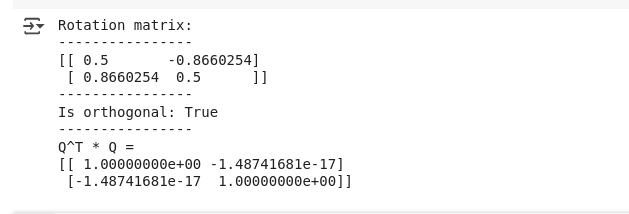Output for orthogonal matrix. Image by Author.

Additionally, we can also verify the function using a non-orthogonal matrix below:

# Test with a non-orthogonal matrix
non_orthogonal = np.array([[1, 2], [3, 4]])
print("\nNon-orthogonal matrix:")
print(non_orthogonal)
print("Is orthogonal:", is_orthogonal(non_orthogonal))

The output confirms the same:

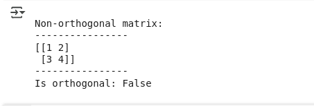
Output for non-orthogonal matrix. Image by Author.

The tolerance parameter accounts for floating-point arithmetic precision. In practice, matrices that are computationally orthogonal (within numerical precision) are acceptable for most applications, even if they’re not mathematically perfect due to rounding errors.

Conclusion

This article explored orthogonal matrices, special square matrices where the transpose equals the inverse, and their remarkable properties that make them essential in data science and numerical computing. We learned how these matrices preserve distances and angles during transformations, examined their applications in PCA, QR decomposition, computer graphics, and signal processing, and discovered practical methods for identifying them using Python implementations.

To deepen your knowledge of linear algebra and its applications in data science, consider enrolling in our Linear Algebra for Data Science course, where you’ll explore more advanced matrix concepts and their implementations in real-world scenarios.