SUMIF() in Excel: A Beginner's Guide

To use SUMIF() in Excel, enter =SUMIF(range, criteria, [sum_range]), where range is the cells to check, criteria is the condition to match, and sum_range is the cells to add up. This lets you total values that meet a specific condition without manually filtering or adding rows by hand.

In this article, we'll break down the SUMIF() syntax in detail, walk through a step-by-step example, compare SUMIF() to related functions like SUMIFS() and COUNTIF(), and cover the mistakes that confuse most beginners.

What Is the SUMIF() Function in Excel?

SUMIF() is an Excel function that adds up numbers, but only the ones that meet a condition you set. In simple words, you tell Excel what to look for, and it adds only the matching values.

A simple SUM() formula adds everything in a range. Whereas SUMIF() is more selective. It checks each cell against your condition, and only adds the ones that pass. If a cell does not match, Excel skips it.

For example, you may use this formula in case:

• You run a shop and want to know how much you made from just one product.
• You track your spending and want the total for one category, like groceries or rent.
• You manage a team and want to add up hours worked by one employee.

SUMIF() is perfect for each case because you are not interested in the total; you want only a slice of it.

SUMIF() Syntax

The SUMIF() formula follows this structure:

=SUMIF(range, criteria, [sum_range])

In this syntax: 

• range: This is the group of cells Excel checks for your condition. It is where Excel looks to decide what matches and what does not. 

• criteria: It tells Excel what to look for in the range. It could be a word, a number, or a symbol like ">100".

• sum_range (optional): This pulls the numbers to add up once it finds a match. If you skip this part, Excel just adds the values in the range itself.

Here’s a quick example to see how the three parts work together:

=SUMIF(A2:A11, "Apples", B2:B11)

In this formula, 

• A2:A10 is the range, since that is where we are looking for Apples. 

• Apples is the criteria, the exact word we want to match. 

• B2:B10 is the sum_range, since that is where the matching sales numbers are.

So we are checking column A for Apples. Every time there is a match, the corresponding number from column B gets added.

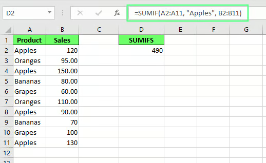
Apply SUMIF() to sum values based on a criteria. Image by Author.

How to Use SUMIF() in Excel

To use SUMIF() in Excel, follow these steps: 

Step 1: Identify the range

We are using the following dataset in our example: 

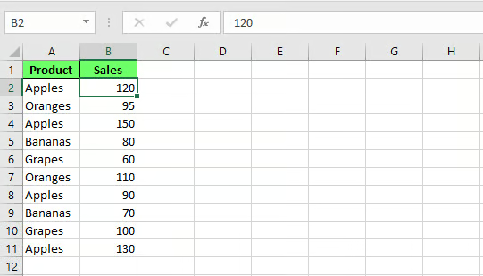
Dataset for SUMIF(). Image by Author.

Select the range where you want to apply the condition. In this case, we want to search for Apples, which is in the Product column, so the range is A2:A11.

Step 2: Set the criteria

Since we want Apples, the criteria is Apples.

You can type the criteria directly into the formula or reference a cell that contains it. Here, we're typing it directly, so it needs to be wrapped in quotation marks since it's text.

Step 3: Set the sum rangeThe sum range is where the actual numbers are. We want to add up sales, so the sum range is B2:B11.

The sum range doesn't have to be the same size or position as the range you searched in. It just needs to line up row by row, so the value SUMIF() adds corresponds to the same row where the criteria matched.

Now, the formula looks like this:

=SUMIF(A2:A11, "Apples", B2:B11)

This is how it will work:

• Row 2 has Apples, so 120 gets added. 
• Row 3 has Oranges, so it gets skipped. 
• Row 4 has Apples again, so 150 gets added. 
• Likewise, rows 8 and 11, so 90 and 130 get added

The final result is 490

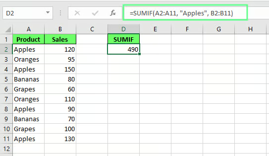
Sum the product sales using SUMIF(). Image by Author.

SUMIF() Examples

Now let's look at a few more situations where SUMIF() can be helpful. Each one uses a slightly different type of criteria, so we will go through them one at a time.

Sum numbers greater than or less than a value

Sometimes we don't want to match a specific word. Instead, we want to catch anything above or below a certain number.

To get the total of all sales greater than 100, we write:

=SUMIF(B2:B11, ">100", B2:B11)

In our table, the values greater than 100 are 120, 150, 110, and 130. Add those up, and we get 510.

Notice that the range and the sum range are the same here. That's because we're checking the numbers themselves, not matching them to a separate column.

For sales less than 50, the formula would be:

=SUMIF(B2:B11, "<50", B2:B11)

In our table, nothing is below 50, so this one returns 0 instead of an error, just no matches.

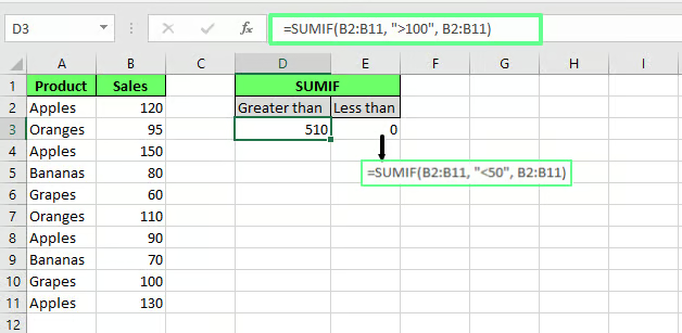
Summing numbers that match greater-than or less-than criteria. Image by Author.

Sum dates

Dates work a bit differently, since Excel stores them as numbers. Every date is a serial number counting from a fixed starting point. This is why we can use comparison symbols with dates too, the same way we did with regular numbers.

Let's say we have a column of order dates in column C, and we want the total sales after March 1, 2026. The formula would look like this:

=SUMIF(C2:C11, ">"&DATE(2026,3,1), B2:B11)

In the screenshot below, I've highlighted the matching dates and the total they add up to.

We use the DATE() function here instead of typing the date directly. This avoids errors, since Excel can read dates differently depending on your regional settings.

If we wanted expenses during a specific month, say March 2026, we'd need two conditions instead of one, since we're checking a range rather than a single point. 

That's actually where SUMIF() reaches its limit — we'll get to that in the comparison section coming up.

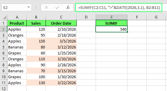
Sum of sales matching the date criteria using SUMIF(). Image by Author.

Use cell references as criteria

So far, we've typed our criteria directly into the formula, like "Apples" or ">100". This works fine, but it's not very flexible. If we want to check a different product, we'd have to edit the formula every time.

A better approach is to reference a cell instead. Suppose cell A6 contains the word Grapes. Our formula would look like this:

=SUMIF(A2:A11, A6, B2:B11)

This sums up all the values of Grapes. Now, if we want to check a different product, we only change what's in A6; no need to touch the formula at all.

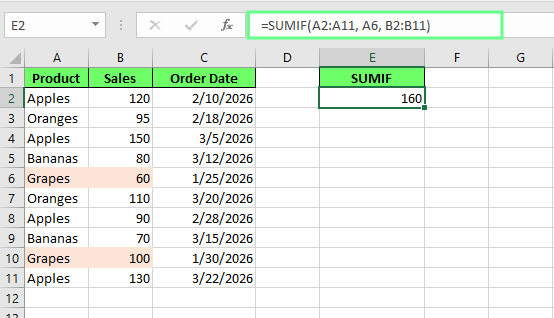
Use cell reference instead of hardcoding the criteria. Image by Author.

How to Use Wildcards with SUMIF()

Wildcards match the pattern if we don't know the exact text. For example, you don't know the exact word but know the word starts with B. 

SUMIF() supports two wildcards: 

• * stands for any number of characters. It could be zero characters, one character, or a hundred characters.

• ? stands for exactly one character.

Let's see how these work with our product table.

Products beginning with "A"

Let’s say we want the total sales for every product that starts with A. Instead of writing four separate formulas for Apples, Apricots, Avocados, and Almonds, one wildcard formula handles all of them:

=SUMIF(A2:A8, "A*", B2:B8)

The asterisk after A tells the formula to match A followed by anything. Every product in our table starting with A gets captured here. That's 120 plus 90 plus 60 plus 75, giving us 345.

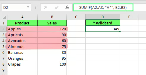
Products starting with the letter A using the * wildcard. Image by Author.

Names containing certain text

Wildcards also work in the middle of a word. Let’s say we want every product that contains “an” somewhere in its name. That catches Bananas and Oranges both. 

For this, the formula becomes:

=SUMIF(A2:A8, "*an*", B2:B8)

The asterisk on both sides means we don't care what comes before or after an. As long as an shows up somewhere in the text, it counts as a match. 

Running this on our table adds up sales from both Bananas and Oranges, giving us 175. 

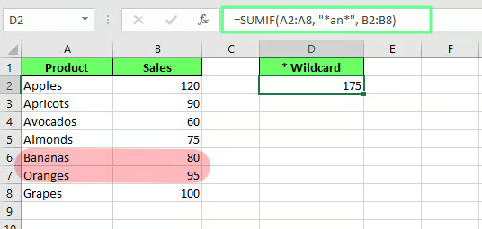
* finds the product containing specific character(s). Image by Author.

When to use ? instead of *

? matches exactly one character. If we have product codes and we only want codes with exactly one digit after the letter A, we'd write:

=SUMIF(A2:A7, "A?", B2:B7)

This matches A1, A2, and A3, but not A10 or A11, since those have two characters after the A, not one.

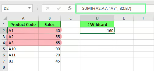
Match the pattern using the ? wildcard. Image by Author.

So:

• Use * when the text length varies. 

• Use ? when you know exactly how many characters to expect.

SUMIF() vs. SUMIFS()

SUMIFS() does the same job as SUMIF(): 

• SUMIF() checks one condition at a time. 

• SUMIFS() checks multiple conditions at once.

Here's a quick comparison.

The syntax of SUMIFS() is:

SUMIFS(sum_range, criteria_range1, criteria1, [criteria_range2, criteria2], …)

The difference in SUMIF() is that the sum_range comes last. In SUMIFS(), it comes first. 

Let's see this with an example. 

In our sales table, we want total sales for Apples, but only where sales were above 100. That's two conditions. 

Unlike SUMIF(), SUMIFS() can handle it. Here’s how: 

=SUMIFS(B2:B11, A2:A11, "Apples", B2:B11, ">100")

Here, B2:B11 is the sum_range, listed first. Then we have our condition pairs: A2:A11 with Apples, and B2:B11 with >100. Excel checks both conditions for every row, and only adds the sales figure when both are true.

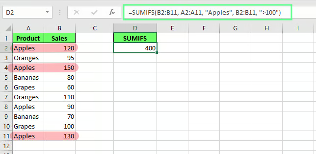
SUMIFS() checks multiple conditions at once. Image by Author.

SUMIF() vs. COUNTIF()

SUMIF() and COUNTIF() look similar, since both check a condition before doing something. But they don't do the same job.

• SUMIF() adds up values that match a condition. 

• COUNTIF() counts how many cells match a condition. 

Here's a quick comparison.

One gives you a total. The other gives you a count. Let's see this side by side, using our original sales table.

Here we want to know two things about Apples. 

1. How much did we sell in total
2. How many times does Apples appear in the list?

For the total sales, we use SUMIF():

=SUMIF(A2:A11, "Apples", B2:B11)

This adds up every sales figure where the product is Apples, giving us 490.

For the count, we use COUNTIF():

=COUNTIF(A2:A11, "Apples")

This counts how many rows have Apples in them, giving us 4.

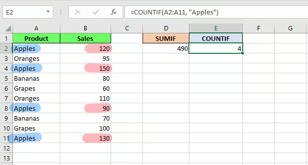
COUNIF() counts the number of instances that appear in a cell. Image by Author.

COUNTIF() only needs a range and a criterion, since there's nothing to add up. But SUMIF() needs a sum range as well, since it's pulling numbers from somewhere to total them.

Common SUMIF() Mistakes

Even with a simple formula, small errors creep in. Here are the mistakes we see most often, along with how to fix each one.

Using the wrong range

This happens when the range and the sum range don't line up row for row. Say your range is A2:A11, but your sum range is B2:B10. Excel now has one row of mismatch, and the totals come out wrong, sometimes without any error message at all.

To fix this: make sure both ranges start and end on the same rows. If your range is A2:A11, your sum range should also run from row 2 to row 11.

Forgetting the sum range

Let's say you want to add up column B, but your condition is checking column A. If you write the formula with only A2:A11 and the criteria, and leave out the sum range, Excel assumes you want to add up column A itself, not column B. The result came out wrong.

To fix this: always include the sum range when the column you're checking is different from the column you're adding. If both columns happen to be the same, you can technically skip it. Still worth adding anyway, just to keep things clear.

Incorrect criteria syntax

Write >100 without quotation marks, and it throws an error. It needs to be written as ">100", with double quotes around it. Single quotes throw an error too.

To fix this: any criteria using text or comparison symbols needs quotation marks. If you're matching an exact number, like the number 100 by itself, you don't need quotes. The moment a symbol or word is part of the criteria, quotes are required.

Numbers stored as text

Sometimes numbers in a spreadsheet look like numbers, but Excel is actually treating them as text. This usually happens when data is imported from another source, like a CSV file or a system export. 

You'll notice this if the numbers are aligned to the left instead of the right, which is Excel's usual way of displaying text.

When this happens, SUMIF() using a comparison like ">100" won't work correctly, since Excel can't compare text values the same way it compares actual numbers.

To fix this: convert the text back into numbers. Go to the Home tab > Number group, and from the dropdown, select General or Number.

Extra spaces in text values

Say one cell has "Apples" and another has "Apples " with a trailing space. To your eyes, they're the same. To SUMIF(), they're not, and the formula won't count them as a match.

To fix this: wrap your formula inside the TRIM() function to remove extra spaces before running it. That way "Apples" and "Apples " are finally treated as the same thing.

SUMIF() Best Practices

A few habits make SUMIF() easier to work with, especially as your spreadsheets grow. Here's what we recommend.

• Use cell references instead of hard-coded criteria: Typing "Apples" directly into a formula works, but it means editing the formula every time you want to check something else. Point to a cell instead, and you only need to change the value in that cell; the formula stays untouched.

• Keep ranges the same size: Your range and your sum range should always cover the same number of rows. If one runs from row 2 to row 11 and the other stops at row 10, the totals won't line up correctly.

• Use Excel Tables for expanding datasets: A regular range like A2:A11 won't automatically include new rows as your data grows. Convert your data into an Excel Table to fix this. As a result, tables expand on their own as you add rows, and your SUMIF() formula grows right along with it; no manual updates needed.

• Test formulas with simple examples: Use five or six rows you already know the answer to, and confirm the formula returns what you expect. This catches mistakes early, before they spread across hundreds of rows.

• Use SUMIFS() when more than one condition is needed: The moment you need to check two things at once, like a product and a date range, switch to SUMIFS(). Trying to force SUMIF() to do that job usually leads to workarounds that are harder to read and easier to break.

Final Thoughts

SUMIF() is the simplest way to add values that meet one condition. Give it a range, a criteria, and a sum range, and it does the rest.

Start with simple conditions, such as matching a product name or a number greater than a certain value. Once that feels comfortable, wildcards and cell references make the formula more flexible without changing how it works underneath.

If you ever find yourself needing to check two things at once, that's your sign to move on to SUMIFS().