Generalized Linear Model (GLM): A Beginner's Guide to Theory and Code

Linear regression is a great first model to try, but it falls short the moment your data doesn't fit a normal distribution.

Let’s say you're trying to predict whether a customer will churn (yes or no outcome). Linear regression doesn't know how to do that. It predicts continuous values, so you end up with outputs like -0.3 or 1.7 for something that can only be 0 or 1. The same problem shows up with count data, like the number of support tickets per hour. Linear regression can predict negative counts, which makes no sense.

Generalized linear models (GLMs) fix this by extending the linear regression to handle different types of outcomes. The core idea is the same - a linear combination of inputs - but with the flexibility to model binary data and other non-normal distributions.

In this article, I'll break down what GLMs are, walk through their three core components, and show you how to fit and interpret them in both Python and R.

But how exactly does linear regression work? Read our guide to Simple Linear Regression to learn its assumptions and diagnostics, and how to interpret the results.

What Is a Generalized Linear Model?

A generalized linear model (GLM) is an extension of linear regression that allows the response variable to follow different probability distributions, not just the normal distribution.

The key thing to remember here is that GLM isn't a single model. It's a framework. Linear regression, logistic regression, and Poisson regression are all GLMs. Each one uses a different distribution and a different way of connecting inputs to outputs, but they all follow the same structure.

Why Generalized Linear Models Are Needed

Standard linear regression makes two big assumptions: your outcome is normally distributed, and the variance stays constant across predictions. If these assumptions don’t hold, you’ll get results that make no sense.

For example, if you’re building a model to predict whether a loan applicant will default, the outcome is binary - 0 or 1. Linear regression doesn't respect that boundary. It can predict -0.2 or 1.4, both of which are impossible.

Count data has the same issue. If you're predicting the number of hospital readmissions per month, linear regression can output negative numbers. You can't have -3 readmissions.

The problem in both cases isn't the linear combination of inputs - that part works fine. The problem is how the model maps those inputs to the output. GLMs solve this by adding a link function that transforms the output to fit the data's natural range. Probabilities stay between 0 and 1. Counts stay non-negative. You’ll see all about it in a bit.

The Three Components of a GLM

Every GLM is built from three parts: a distribution, a linear predictor, and a link function. Let me go through each.

Random component (distribution)

The random component defines what kind of data your response variable produces. In other words, it picks the probability distribution that best describes your outcome.

Linear regression assumes a normal distribution, so the outcome is continuous and symmetric around the mean. But not all data works that way.

If your outcome is binary (yes/no, 0/1), you'd use a binomial distribution. If you're modeling count data - like the number of errors per day - a Poisson distribution is the better fit.

The distribution you choose controls everything else in the model.

Systematic component (linear predictor)

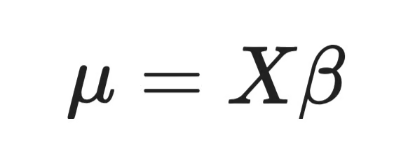
The systematic component is the part you already know from linear regression. It's a linear combination of your input variables:

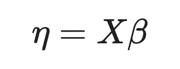
Systematic component

Where X is your matrix of input features and β is the vector of coefficients. You multiply each feature by its weight and add them up.

This part doesn't change across different GLMs. In other words, whether you're fitting a logistic regression or a Poisson regression, the linear predictor looks the same.

Link function

The link function connects the linear predictor to the expected value of the response variable. It's the piece that makes GLMs flexible.

Without a link function, the linear predictor outputs values from negative infinity to positive infinity. That's fine for continuous outcomes, but not for probabilities or counts. The link function transforms the output so it sits in the right range for your chosen distribution.

For example, logistic regression uses the logit link, which maps a linear predictor that can be any real number to a probability between 0 and 1. Poisson regression uses the log link, which makes sure predictions are always positive.

The full GLM equation combines all three components:

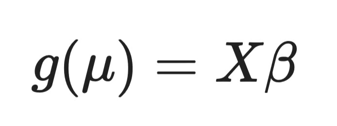
GLM equation

Where g() is the link function and μ is the expected value of the response. The distribution defines what μ means, the linear predictor computes Xβ, and the link function bridges the two.

Common Link Functions (With Intuition)

The link function determines how the linear predictor converts to your outcome. Different data types need different transformations, and each GLM type has a default link function that pairs with its distribution.

Identity link

The identity link is the simplest - it does nothing. The linear predictor equals the expected value of the response:

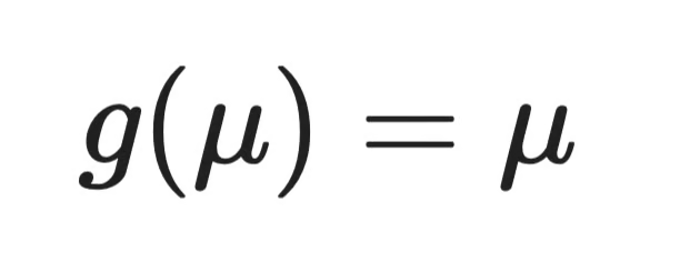
Identity link

This is what linear regression uses. Your inputs combine into a weighted sum, and that sum is the prediction. There is no transformation needed, because the outcome can take any continuous value.

Logit link

The logit link takes a probability (between 0 and 1) and maps it to the entire real number line:

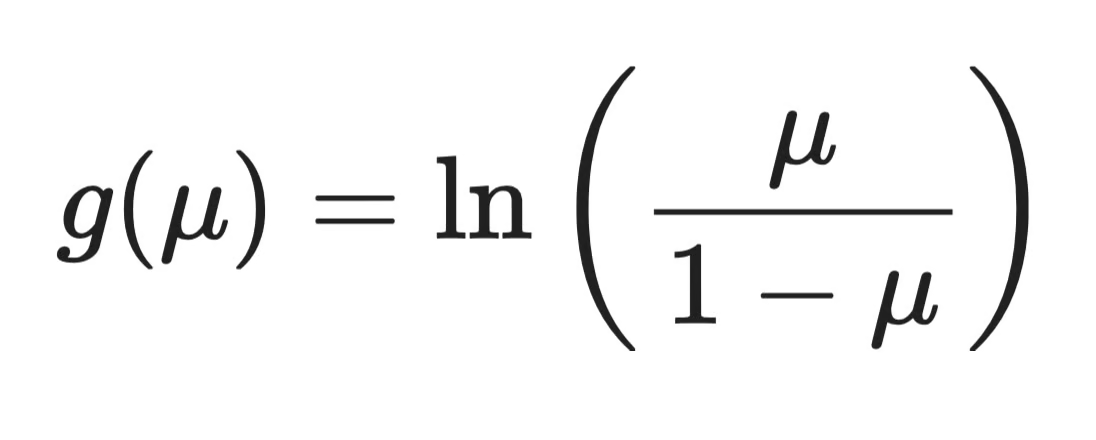
Logit link

This is what logistic regression uses. The linear predictor can output any value from negative infinity to positive infinity, but after the inverse transformation, the prediction always sits between 0 and 1. That ratio inside the logarithm - μ/(1-μ) - is called the odds, and the logarithm of the odds is the log-odds. So when you interpret logistic regression coefficients, you're working in log-odds space.

Log link

The log link takes the natural logarithm of the expected value:

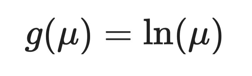
Log link

This is what Poisson regression uses. The linear predictor can be any real number, but after you exponentiate it back (the inverse), the prediction is always positive. That's exactly what you need for count data as you can't have negative events.

Examples of Generalized Linear Models

GLMs can feel abstract until you see them as models you already know. Linear regression, logistic regression, and Poisson regression are all GLMs. The only difference is that each uses a different combination of distribution and link function.

Linear regression as a GLM

Linear regression is the simplest GLM. The response follows a normal distribution, and the link function is the identity link, meaning no transformation at all.

Linear regression as a GLM

The linear predictor directly equals the expected outcome. This is the GLM you've been using all along, just without calling it one.

Logistic regression

Logistic regression models binary outcomes using a binomial distribution and a logit link.

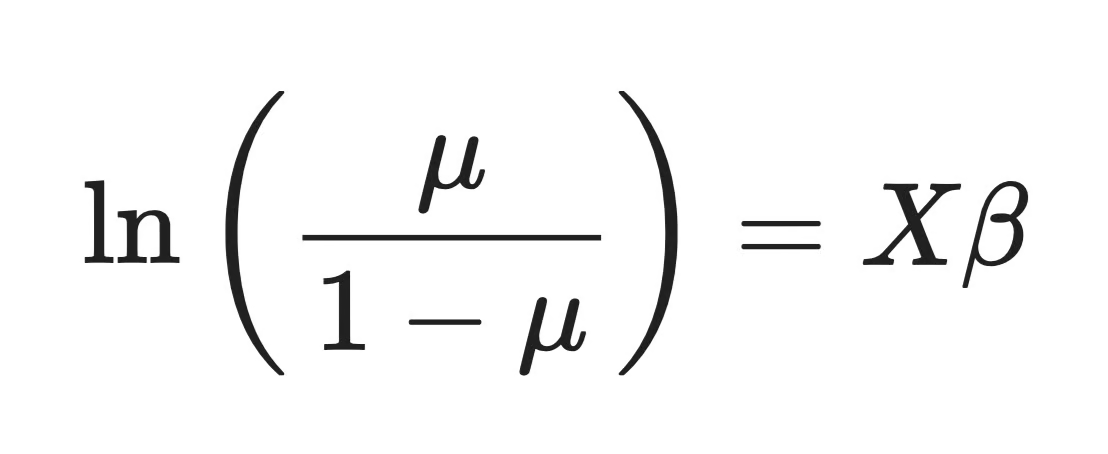
Logistic regression as a GLM

The left side is the log-odds of the event. The right side is your standard linear combination of inputs. The logit link makes sure predictions map to probabilities between 0 and 1, no matter how large or small Xβ gets.

Poisson regression

Poisson regression models count data using a Poisson distribution and a log link.

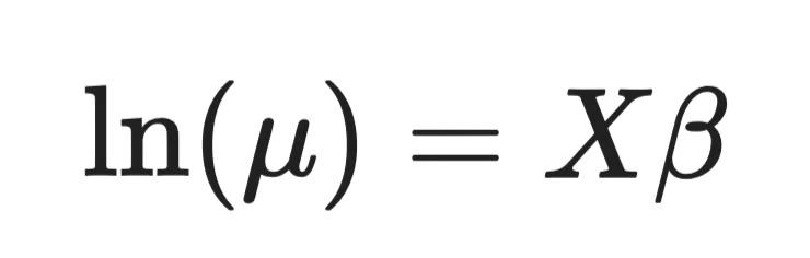
Poisson regression as a GLM

The log of the expected count equals the linear predictor. If you exponentiate both sides, you get μ = e^(Xβ), which is always positive - exactly what counts require.

How GLMs Are Trained

GLMs don't use ordinary least squares like linear regression. Instead, they rely on maximum likelihood estimation (MLE).

The idea is straightforward. MLE finds the set of coefficients that makes your observed data most probable under the chosen distribution. For a logistic regression, it finds the coefficients that make the observed 0s and 1s most likely given a binomial model. For Poisson regression, it finds the coefficients that best explain the observed counts.

There's no closed-form solution for most GLMs, so the optimization is iterative. The algorithm starts with an initial guess for the coefficients, evaluates how well they fit the data, adjusts them, and repeats until the estimates converge.

The most common method is iteratively reweighted least squares (IRLS), which recasts the MLE problem as a sequence of weighted linear regressions. Gradient-based methods also work, as they compute the direction of steepest improvement and step toward it. Libraries like statsmodels and R's glm() do all of this behind the scenes, so you don't need to implement the solver yourself.

The thing to remember is that you choose the distribution and link function, and the optimizer finds the best coefficients. That's the idea - now let me show you how it works in practice.

Generalized Linear Models in Python and R

In this section, I'll walk through logistic regression and Poisson regression in both Python and R using the same dataset - a simulated employee attrition dataset with columns for salary, years of experience, overtime hours, whether the employee left (binary), and number of sick days taken (count).

The dataset

I’ll create the mentioned dataset in Python, and then use it for calculations in both Python and R:

import numpy as np
import pandas as pd

np.random.seed(42)
n = 500

# Employee dataset
df = pd.DataFrame({
    "salary": np.random.normal(55000, 12000, n).astype(int),
    "experience_years": np.random.poisson(5, n),
    "overtime_hours": np.random.poisson(8, n),
})

# Simulate binary outcome: left the company
prob_left = 1 / (1 + np.exp(-(
    -2 + -0.00003 * df["salary"] + -0.05 * df["experience_years"] + 0.12 * df["overtime_hours"]
)))
df["left"] = np.random.binomial(1, prob_left)

# Simulate count outcome: sick days per year
df["sick_days"] = np.random.poisson(
    np.exp(1.2 + 0.00001 * df["salary"] + 0.02 * df["overtime_hours"])
)

# Save to use later in R
df.to_csv("data.csv", index=False)

df.head()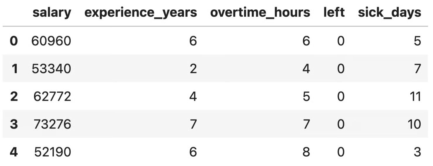

Sample employee attrition dataset

Python implementation

Python gives you two main options for GLMs: statsmodels and scikit-learn. I'll use statsmodels here because it gives you a full statistical summary, including coefficients, p-values, and confidence intervals. You’ll need these when you're interpreting a GLM.

This is how you can fit a logistic regression to predict whether an employee left:

import statsmodels.api as sm

X = sm.add_constant(df[["salary", "experience_years", "overtime_hours"]])
logit_model = sm.GLM(df["left"], X, family=sm.families.Binomial())
logit_results = logit_model.fit()

print(logit_results.summary())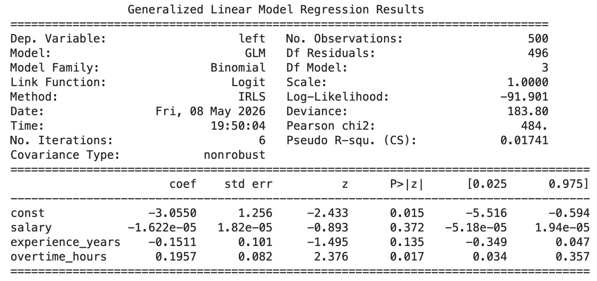

GLM logistic regression results

The key line is sm.families.Binomial(). This sets both the distribution (binomial) and the default link function (logit) in one argument. You don't need to specify the link separately unless you want a non-default one.

Now let's fit a Poisson regression on the same dataset to predict sick days:

poisson_model = sm.GLM(df["sick_days"], X, family=sm.families.Poisson())
poisson_results = poisson_model.fit()

print(poisson_results.summary())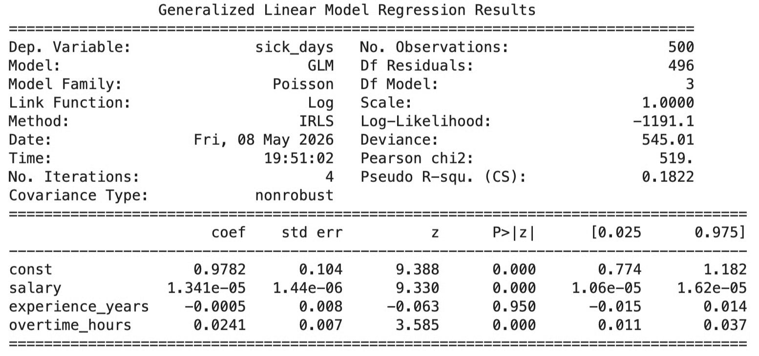

GLM Poisson regression results

You just need to swap Binomial() for Poisson() and the model uses a Poisson distribution with a log link. The output table looks the same, but the interpretation changes because the link function changed.

Let me now visualize the predicted probabilities from the logistic regression against overtime hours:

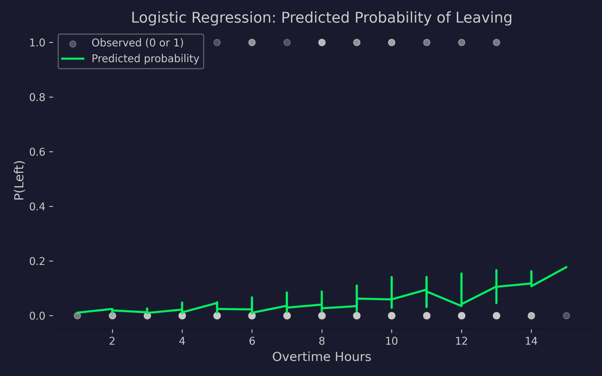
Predicted probabilities for leaving the company against overtime hours

The chart shows overtime hours on the x-axis against the probability of leaving on the y-axis. The gray dots are the actual outcomes - either 0 (stayed) or 1 (left). The green curve is the model's predicted probability. As overtime hours increase, the predicted probability of leaving rises, but it never drops below 0 or exceeds 1. That's the logit link function at work - it squashes the linear predictor into a valid probability range no matter how extreme the input values get.

R implementation

R's built-in glm() function follows the same logic but with a different syntax. The family argument sets the distribution and link function, and you define the model with R's formula interface.

Here's the same logistic regression in R:

# Read the dataset
df <- read.csv("data.csv")

# Fit logistic regression
logit_model <- glm(left ~ salary + experience_years + overtime_hours,
                   data = df,
                   family = binomial(link = "logit"))
summary(logit_model)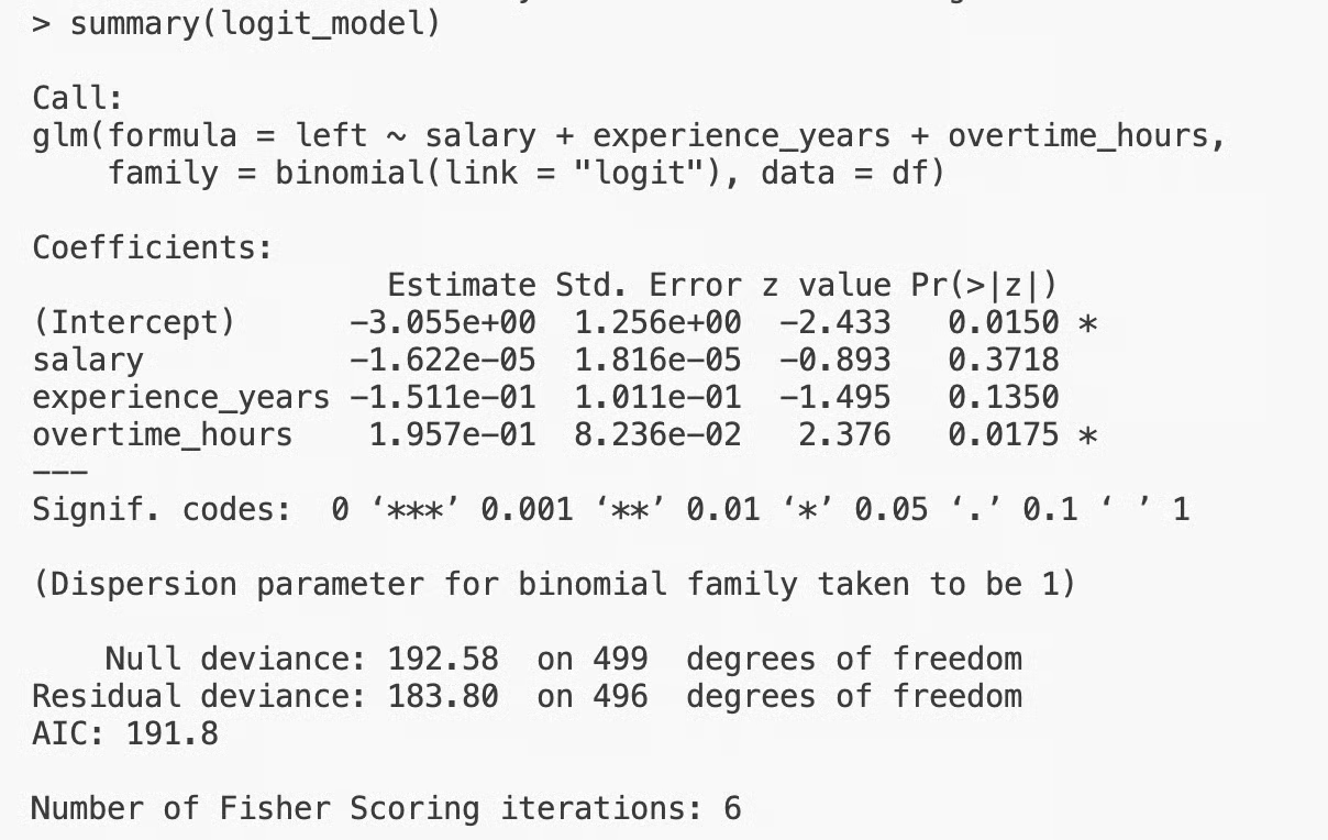

GLM logistic regression in R

The formula left ~ salary + experience_years + overtime_hours tells R what to predict and which inputs to use. The family = binomial(link = "logit") part sets the distribution and link. You can shorten this to family = binomial() since logit is the default link for the binomial family.

Poisson regression is mostly the same:

poisson_model <- glm(sick_days ~ salary + experience_years + overtime_hours,
                     data = df,
                     family = poisson(link = "log"))
summary(poisson_model)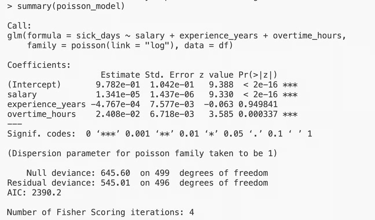

GLM Poisson regression in R

You just need to change binomial() for poisson(), change the response variable, and you're done.

How distribution and link are specified

Both languages use the same approach - you pass a family/distribution argument that combines the distribution and its default link function:

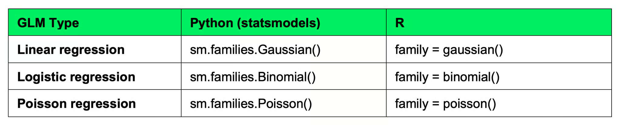
Specifying distribution and link in Python and R

Each family has a default link, but you can override it. In Python, you can pass a link object: sm.families.Binomial(link=sm.families.links.Probit()). In R, just change the link argument: family = binomial(link = "probit").

For most use cases, the default link is the right choice.

Interpreting GLM Coefficients

GLM coefficients don't mean the same thing across different model types. The link function changes how you interpret them.

In linear regression, interpretation is easy. A coefficient of 500 on experience_years means each extra year of experience adds 500 to the predicted salary. The identity link means coefficients map directly to the outcome.

Logistic regression is different. The logit link means coefficients are in log-odds space. A coefficient of 0.12 on overtime_hours doesn't mean the probability of leaving goes up by 0.12. It means the log-odds of leaving increase by 0.12 for each additional overtime hour. To get something more interpretable, exponentiate the coefficient: e^0.12 ≈ 1.127. This gives you an odds ratio. Each extra overtime hour multiplies the odds of leaving by about 1.13.

Poisson regression coefficients work through the log link. A coefficient of 0.02 on overtime_hours means each additional hour increases the log of the expected count by 0.02. When you exponentiate it: e^0.02 ≈ 1.02, you’ll see each extra overtime hour multiplies the expected number of sick days by about 1.02.

The pattern is to always apply the inverse of the link function to move from coefficient space back to the outcome space.

When to Use a Generalized Linear Model

Picking the right GLM comes down to one question: what does your outcome variable look like?

If your outcome is binary (yes/no, 0/1, pass/fail), use logistic regression. Binomial distribution, logit link. This covers classification tasks like predicting churn, fraud detection, disease classification (has or doesn’t have), or whether a patient will respond to treatment.

If your outcome is a count (number of events in a time window), use Poisson regression. Poisson distribution, log link. This fits problems like predicting the number of website visits per hour or insurance claims per year.

If your outcome is continuous and roughly normal (revenue, test scores), standard linear regression works just fine. Normal distribution, identity link. This is the GLM you already know.

Always start with the outcome variable, match it to a distribution, and then the link function follows.

Common Mistakes With GLMs

Here are some common mistakes you should avoid when working with GLMs.

Choosing the wrong distribution

This is the most common mistake. If your outcome is a count and you fit a linear regression, you'll get negative predictions. If it's binary and you use Poisson, the model won't make sense. Always look at your outcome variable first and pick the distribution that matches it.

Misunderstanding the link function

The link function transforms the relationship between inputs and output. A logistic regression coefficient of 0.5 doesn't mean "the probability goes up by 0.5." It means the log-odds go up by 0.5. Forgetting the transformation leads to wrong conclusions about effect sizes and variable importance.

Misinterpreting coefficients across model types

Coefficients in a Poisson regression aren't comparable to coefficients in a logistic regression, even if the numbers look similar. A coefficient of 0.3 means something different depending on whether it's passed through a log link or a logit link. Always interpret coefficients in the context of the specific model you're using.

Ignoring model assumptions

GLMs are more flexible than linear regression, but they still have assumptions. Poisson regression assumes the mean equals the variance - if your count data has much more variance than the mean, the model's standard errors will be too small and your p-values will be misleading. Logistic regression assumes observations are independent.

To overcome this, after fitting any GLM, check the residuals and look for patterns that suggest a bad fit.

Conclusion

GLMs give you a structured way to go beyond linear regression but still follow its fundamental logic. The idea of a linear combination of inputs stays the same, but the distribution and link function change to fit the data you’re working with.

There are three components behind GLMs. Once you know how to pick the right distribution, set up the linear predictor, and apply the correct link function, you can handle binary outcomes, counts, and continuous data with the same mental model.

The best next step is to try it. Pick a dataset with a non-normal outcome, fit a GLM in Python or R, and practice interpreting the coefficients through the link function. Use a dataset you care about, and every bit of theory discussed will click in a matter of minutes.

If you want to go beyond linear regression and GLMs, enroll in our Machine Learning Scientist in Python track. It shows you everything you need to get job-ready in 2026.