Waterfall Chart Excel: A Step-By-Step Guide

A waterfall chart shows how a value changes step by step from a starting point to a final result. It clearly displays how different increases and decreases affect the total. 

This makes it useful for explaining changes in revenue, budget adjustments, profit breakdowns, or any situation where values build on one another.

In this guide, we will walk through how to create a waterfall chart step by step. 

How to Create a Waterfall Chart in Excel

To create a waterfall chart in Excel, follow these steps: 

Step 1: Structure the data 

Create a simple two-column table with positive (increases) and negative (decreases) values: 

1. In Column A, enter the category names. These represent the steps in your calculation.
2. In Column B, enter the values for each step.

Place the starting value at the top and the final value at the bottom. The rows in between should only contain the changes.

Do not calculate running totals in the table. Excel calculates them inside the chart.

Here is how the data should look:

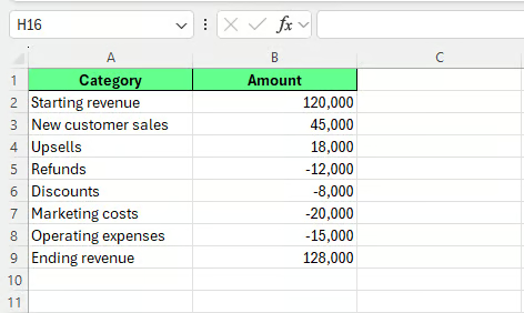
Create a dataset for a waterfall chart. Image by Author.

Step 2: Insert the waterfall chart

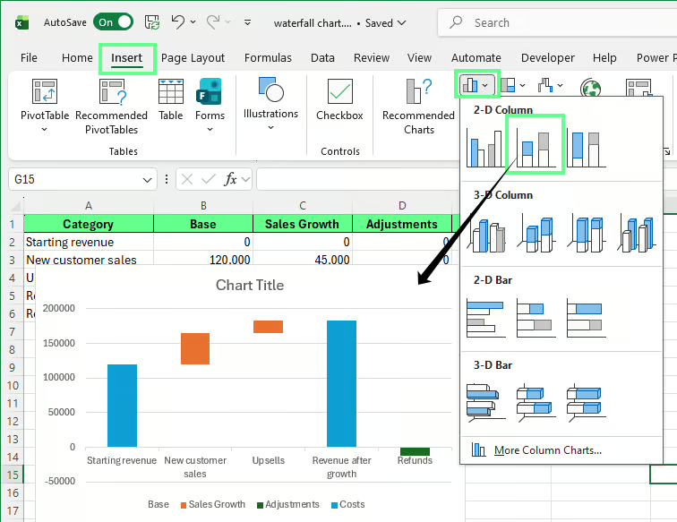
To insert the waterfall chart: 

1. Select both columns, including the headers
2. Go to the Insert tab in the ribbon
3. In the Charts group, select Waterfall
4. Choose Waterfall Chart.

Excel will create the chart based on your data.

At this stage, the chart may not look completely correct. Some columns may appear as regular increases instead of totals.

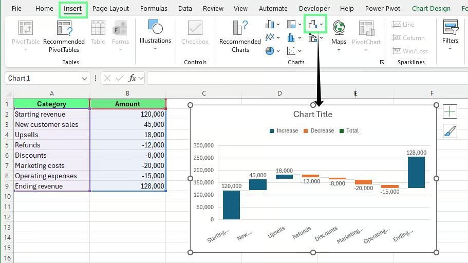
Insert a waterfall chart into the sheet. Image by Author.

Step 3: Set totals correctly

To set totals: 

1. Click any column in the chart
2. Click again on the bar that represents the total (for example, Starting Revenue)
3. Right-click the bar and select Set as Total

Repeat the same process for the Net Profit column.

If your chart includes intermediate totals such as Subtotal or Operating Profit, mark those as totals as well.

When a column is set as a total, it anchors to zero and uses the total color. It no longer floats up or down in the chart.

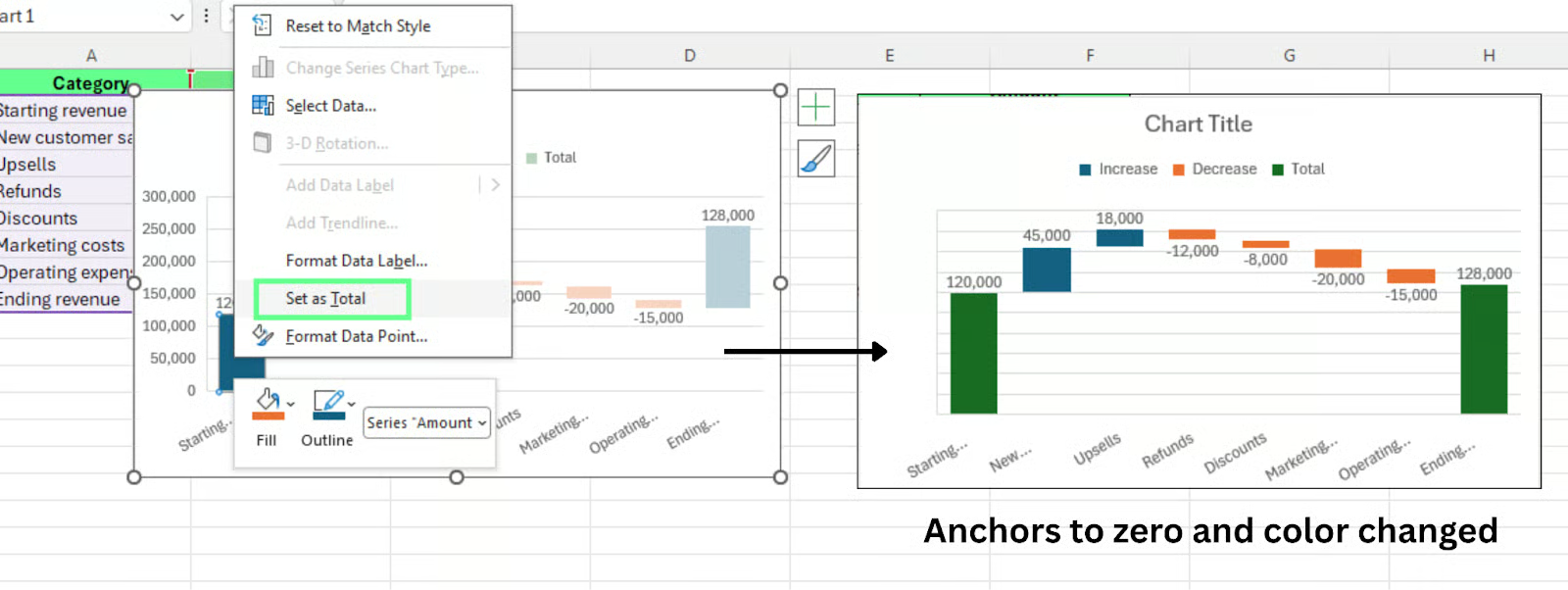
Set numbers as total. Image by Author.

Excel treats every value as a change by default. It does not automatically detect totals. You need to mark total columns manually. If you skip this step, totals will appear to float rather than anchor to zero.

Step 4: Format the chart

After setting totals, you can improve the chart’s appearance, too.

Change bar colors

Excel uses default colors for increases, decreases, and totals. To customize them: 

1. Click any column in the chart
2. Right-click and select Format Legend Entry
3. Open the Fill section
4. Choose a color for each bar type

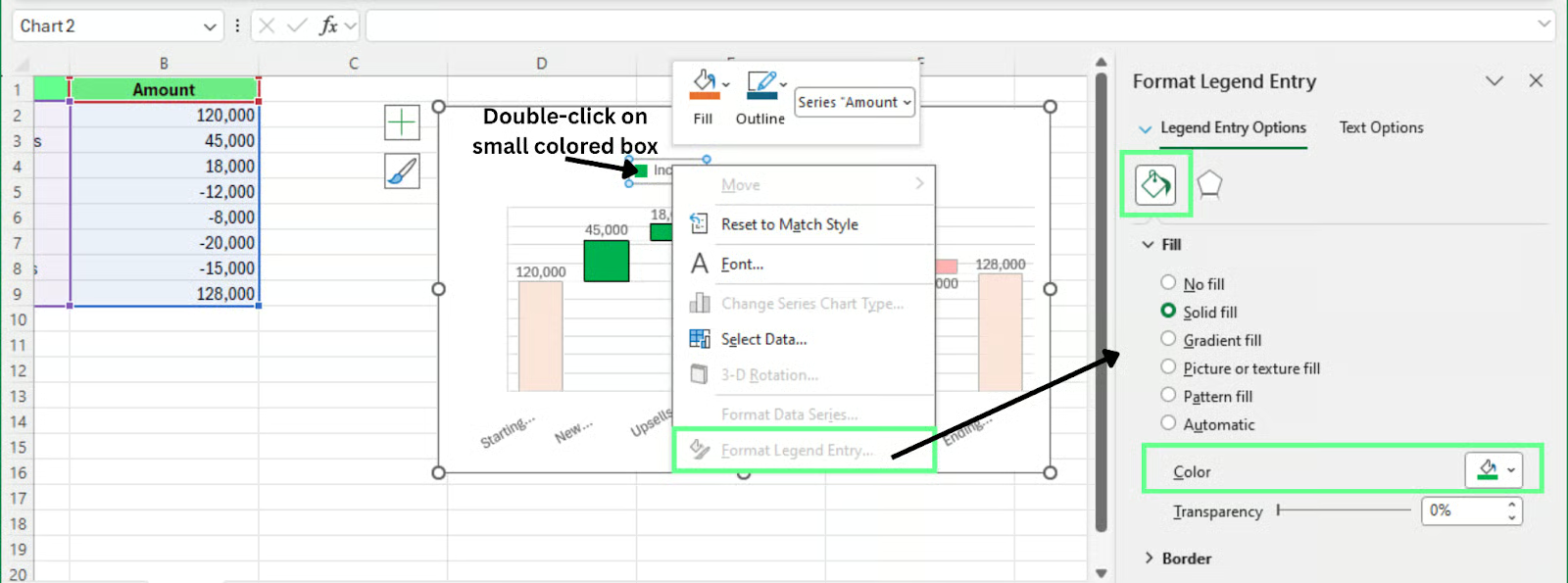Color the bar in the waterfall chart. Image by Author.

Add and adjust chart elements

To add or edit chart elements:

1. Click the chart
2. Click the + icon next to it
3. Select the elements you want to add or adjust

You can also double-click the chart title and rename it.

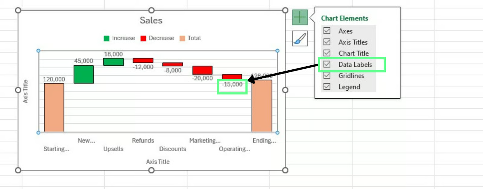
Adjust the waterfall chart. Image by Author.

If the labels overlap:

1. Right-click a label
2. Select Format Data Labels
3. Change the label position

You can also adjust the number format in the Number section.

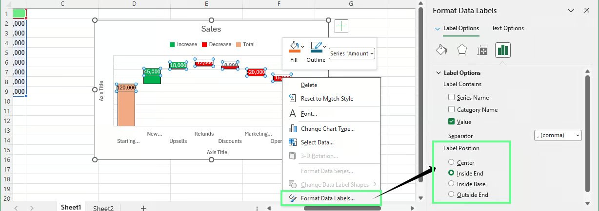
Adjust the label position inthe waterfall chart. Image by Author.

Tip: Use simple number formats and avoid unnecessary decimal places.

Show connector lines

Connector lines link the bars and show how the values move from one step to the next. To enable them:

1. Click any bar
2. Open Format Data Series
3. Check Show connector lines

Connector lines make the flow between steps easier to follow. If they are hard to see, remove the gridlines to reduce visual clutter.

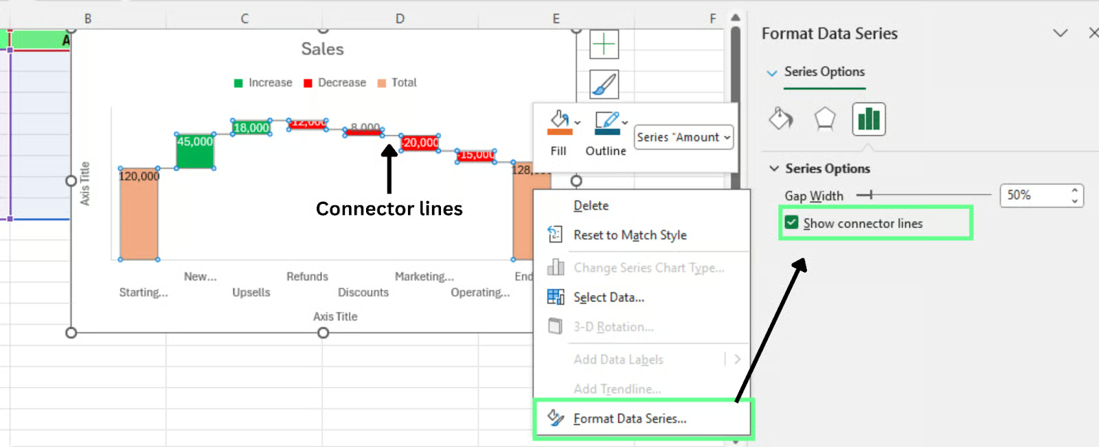
Enable the connector lines in the waterfall chart. Image by Author

Fixing Common Waterfall Chart Issues

Even if you follow the steps correctly, small issues can still appear in the chart. Here are the most common problems and how to fix them.

1. Totals are not anchored to zero

This usually happens when a total column is not marked as a total.

To fix this:

• Right-click the column and select Set as Total
• Check both the first and last bars in the chart

2. Bars appear in the wrong order

This happens when the order of the rows in the worksheet is incorrect. Excel follows the exact sequence of the data.

To fix this:

• Reorder the rows in the worksheet. The chart updates automatically once the order changes.

3. All bars have the same color

This occurs when Excel is not using different formats for increases and decreases.

To fix this:

• Right-click any bar and select Format Data Series
• Enable different colors for positive and negative values
• You can also adjust the colors manually if needed

4. Labels overlap or are hard to read

This usually happens when the chart is too small or when there are many values.

To fix this:

• Resize the chart
• Change the label position
• Simplify the number formatting

Sometimes removing extra detail makes the chart easier to read.

5. The chart does not update after editing data

This happens when the chart range does not include the new rows.

To fix this:

• Right-click the chart and select Select Data
• In the Select Data Source window, expand the data range in your worksheet
• Click OK to update the chart

Tip: Convert your dataset into an Excel table first. Charts linked to tables update automatically when new rows are added.

How to Create a Stacked Waterfall Chart in Excel

A stacked waterfall chart shows how a value changes while also breaking each step into multiple contributors. To create one using a stacked column chart, follow this three-step high-level setup approach: 

Step 1: Arrange the data

Structure your data with separate columns for each component. Each column represents one contributor to the change. For example:

• Online sales
• Retail sales
• Subscriptions

You also need a Base column. This column controls where each stack begins and helps position the bars correctly.

Here is how my dataset looks:

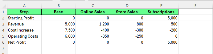
Create a dataset for a stacked waterfall chart. Image by Author.

Step 2: Insert a stacked column chart

To create the stacked chart:

1. Select the full dataset, including the headers
2. Go to the Insert tab
3. Open the Column or Bar Chart menu
4. Select 2-D Column → Stacked Column

Excel will insert a stacked column chart based on your data.

Insert a stacked column chart to create a waterfall chart. Image by Author.

Step 3: Hide the base series

The Base series is only used to position the stacks. We hide it so the bars appear to float like a waterfall chart.

To hide it: 

1. Click any bar from the Base series
2. Right-click and select Format Data Series
3. Set Fill to No Fill
4. Set Border to No Line

After hiding the Base series, the remaining bars will appear to rise and fall from the previous step.

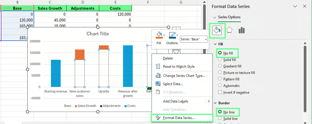
Remove the base series to create a waterfall effect. Image by Author.

Native Excel limitations

Excel’s built-in waterfall chart does not support stacking. Each step can only display one value. Because of this, stacked waterfall charts:

• Require manual setup
• Do not update automatically
• Are harder to maintain

This method is useful when you need to show detailed contributors within each step of the change.

Standard vs. stacked waterfall chart 

In a standard waterfall chart, each step contains one value. A stacked waterfall splits the bar into parts. Each part represents a different component of the change.

For example, a revenue increase may come from:

• Online sales
• Retail sales
• Subscriptions

All three appear inside the same bar. Together, they form the total change. 

This allows the chart to answer two things at once:

• Did the value increase or decrease?
• What contributed to that change?

How to Create a Dynamic Waterfall Chart in Excel

A dynamic waterfall chart is a chart that updates automatically when the underlying data changes. Instead of using a fixed cell range, it is linked to data that can expand or update, such as an Excel table.

This is helpful when the data changes frequently. For example, if you update financial results every month or add new rows to track performance, the chart adjusts automatically without rebuilding it.

To create a dynamic chart, connect your chart to an Excel table using these steps:

1. Convert your data into a table. Select the dataset and press Ctrl + T.
2. Insert a waterfall chart using the table data.
3. Use formulas for totals or changes if needed, and reference the table columns instead of fixed cells.

Once the chart is linked to the table, Excel updates the chart automatically when new rows are added or values change.

Tip: Keep the table structure consistent. Changing column order or inserting blank rows can break the chart logic.

Final Thoughts 

Once you are comfortable with the basics of building a waterfall chart, focus on improving how you present the chart. Clear labels, correct totals, and simple formatting make the biggest difference when someone reads your chart.

If you work with reports that update frequently, connect your chart to an Excel table so it updates automatically. This small step can save time and prevent errors when the data changes.

Strengthen your broader data visualization and Excel skills. Our Data Visualization in Excel course is a good next step if you want to build better charts and dashboards. 

For quick references while working, our Data Visualization Cheat Sheet and Excel Formulas Cheat Sheet can also help you work faster when preparing your data and charts.