Stepwise Regression: Choose Predictors One Step at a Time

Have you ever looked at a regression dataset with 20 predictors and wondered which ones to include in the model?

If you add them all in, the model will likely fit noise along with the signal. If you choose by hand, two analysts can look at the same data and come up with two different models. And needless to say, even with only 20 predictors, there are over a million possible subsets to compare.

Stepwise regression automates this search, as it adds or removes one predictor at a time based on a statistical criterion like a p-value or AIC. It's widely taught and used, but it also has some statistical limitations, so you shouldn't treat it as a default feature-selection method.

In this article, I'll walk you through the three main approaches: forward selection, backward elimination, and bidirectional stepwise selection.

Looking for more feature selection techniques? Read our Python Feature Selection Tutorial for a beginner-friendly introduction to the subject.

What Is Stepwise Regression?

Stepwise regression is an automated procedure for choosing which predictors go into a regression model.

It doesn't fit one model, but instead, it fits a sequence of candidate models, and at each step it adds or removes a predictor based on a selection criterion. The search ends when no further change improves the model by that criterion.

Imagine you want to predict how much a customer spends per year. You have five candidate predictors:

• income

• age

• education

• location

• years_experience

Stepwise regression could start with income, then test whether age improves the model, then education, and so on. The final model might keep only income and education if the other three don't improve the criterion enough.

One key distinction to remember is that stepwise regression isn't a separate type of regression model.

It's a variable selection procedure you run on top of a model you already know, usually linear regression. The output is still an ordinary regression model, stepwise only decides which predictors it gets.

How Stepwise Regression Works

Every stepwise procedure goes through the same loop:

1. Start with an initial model: It can have no predictors, all of them, or something in between
2. Propose a change: Add one predictor or remove one
3. Score the new model: Evaluate it with a predefined criterion
4. Keep or reject the change: Keep it only if the criterion says the new model is better
5. Repeat: Go back to step 2 until no remaining change improves the model

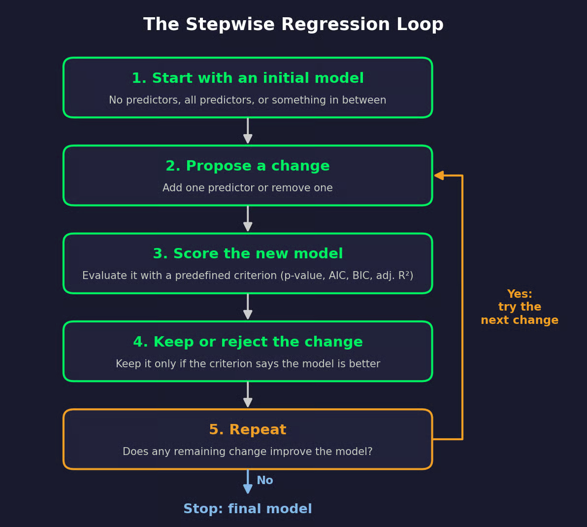
Stepwise regression loop

The algorithm never looks more than one step ahead. It only asks whether the next single change helps.

The criterion decides what "better" means. These are the four you'll see most often:

1. P-values: A predictor enters the model if its p-value falls below an entry threshold, and leaves if it rises above a removal threshold
2. AIC: The Akaike information criterion rewards model fit and penalizes each extra parameter, and lower values are better
3. BIC: The Bayesian information criterion works like AIC, but its penalty per parameter grows with sample size, so it usually ends up with smaller models
4. Adjusted R-squared: Regular R-squared never decreases when you add a predictor, so the adjusted version corrects for the number of predictors, and higher values are better

The exact procedure depends on the search direction and the criterion. Forward selection only adds predictors, backward elimination only removes them, and bidirectional selection does both. And the same dataset can produce different final models depending on which criterion you choose.

So when someone says they ran stepwise regression, the first two questions to ask are which direction and which criterion.

Types of Stepwise Regression

There are three types of stepwise regression, and they differ in one thing - the direction of the search.

Forward selection

Forward selection starts small and builds from there.

You begin with an intercept-only model, or with a couple of predictors you want in the model no matter what. The algorithm then fits one candidate model per remaining predictor, each with that one predictor added. The predictor that improves the criterion the most enters the model.

The loop then runs again, with the bigger model as the new base. It stops when no remaining predictor meets the selection rule, for example when no addition lowers AIC.

Forward selection can start even when you have more candidate predictors than observations, because it never needs to fit the full model. The catch is that once a predictor is in, it stays in, even if later additions make it redundant.

Backward elimination

Backward elimination goes the other way.

You start with the full model, which includes every candidate predictor. The algorithm tries to remove each predictor one at a time and drops the one whose removal improves the criterion the most. Then it refits the smaller model and repeats. The search stops when no removal improves the criterion.

This approach means that the full model must be estimable. You need more observations than parameters, and no predictor can be an exact linear combination of the others. If you have 50 predictors and 40 rows, backward elimination can't even start.

And it has the mirror-image problem of forward selection meaning that once a predictor is out, it stays out.

Bidirectional stepwise selection

Bidirectional selection combines both. After each addition, the algorithm checks whether any predictor already in the model should now come out.

This matters because the value of a predictor depends on what else is in the model. Let's say bedrooms enters first because it's correlated with house size. When square_feet enters later, bedrooms may add almost nothing to it. Bidirectional selection can remove it at that point, while forward selection would keep it.

The price is more model fits per step. You can start bidirectional selection from an empty model or a full one.

Here's how the three compare:

Types of stepwise regressions

Stepwise Regression Example

Let's make this more tangible.

I generated a synthetic dataset of 200 houses and want to predict price from five candidate predictors:

• square_feet

• bedrooms

• age_years

• distance_km (distance from the city center)

• lot_size_sqft

I'll use forward selection with AIC as the criterion, where lower AIC is better. You'll see the same data again in the Python section.

The intercept-only model has an AIC of 5057.0. Here's what each step looks like - every cell shows the AIC you'd get by adding that predictor to the current model:

AIC comparison

This is what happens at each step:

• Step 1: square_feet reduces AIC by about 102 points, so it enters first. bedrooms comes in second place because it's correlated with house size

• Step 2: distance_km gives the biggest drop. bedrooms now barely helps, since square_feet already has most of its information

• Step 3: age_years enters

• Step 4: lot_size_sqft lowers AIC by only 1.6 points, but lower is lower, so it enters

• Step 5: Adding bedrooms would raise AIC to 4840.8, so the search stops

The final model uses square_feet, distance_km, age_years, and lot_size_sqft.

That's a reasonable result. I generated the data so that bedrooms has no direct effect on price, and the procedure left it out.

If you run backward elimination on the same data, it starts from the full model at 4840.8, drops bedrooms, and stops at the same four predictors. Forward and backward won't always agree, but here they do.

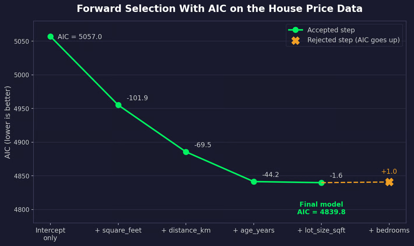
AIC of the current model after each forward selection step

How Variables Are Selected in Stepwise Regression

The search direction decides how the algorithm behaves. The criterion decides when it stops.

P-value-based selection

This is the oldest approach, and it uses two thresholds:

1. Entry threshold: A candidate enters the model if its p-value is below this value, for example 0.05
2. Removal threshold: A predictor leaves the model if its p-value rises above this value, for example 0.10

The removal threshold is usually set higher than the entry threshold, so a predictor doesn't go in and out of the model on every step. Both values are conventions, not rules.

Every p-value assumes you ran one test you planned in advance. Stepwise runs a batch of tests at every step and keeps the smallest p-value. If you run 20 independent tests at 0.05 on predictors with no effect at all, the chance that at least one looks significant is 1 − 0.95^20, which is about 64%. The selected predictors will look stronger than they are, and I'll cover why in the problems section.

In the house price example, lot_size_sqft has a p-value of about 0.063 at step 4. With a 0.05 entry threshold, forward selection stops at three predictors.

AIC

The Akaike information criterion balances model fit against complexity:

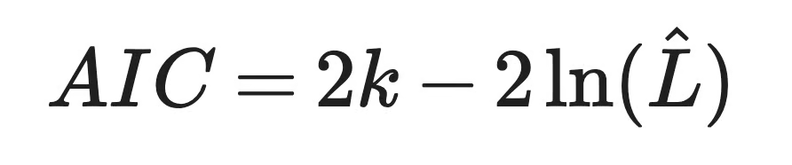
AIC formula

Here, k is the number of estimated parameters and L̂ is the maximized likelihood of the model. The second term rewards fit, and the first term charges 2 points for every parameter.

A new predictor never lowers the likelihood, so the fit term can only improve. The question is whether it improves by more than the 2-point charge. For a single added parameter, that's the same as a likelihood ratio test at a p-value threshold of about 0.157.

That's why lot_size_sqft got in under AIC but not under the 0.05 p-value rule. AIC is more lenient, and it tends to keep weaker predictors that help prediction.

BIC

The Bayesian information criterion has the same structure, with a different penalty:

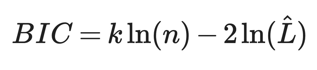
BIC formula

In this formula, n is the number of observations. Each parameter now costs ln(n) points instead of 2, so BIC penalizes complexity more than AIC once you have 8 or more observations. And the gap grows with sample size.

With 200 houses, ln(200) is about 5.3, which works out to an implicit p-value threshold of about 0.021 for one added parameter. Forward selection with BIC on the house data stops at three predictors and leaves lot_size_sqft out.

Adjusted R-squared

Ordinary R-squared is useless as a selection criterion.

It never decreases when you add a predictor to a linear regression model, even a column of random noise. If you select by R-squared, the full model is always the best.

Adjusted R-squared adds a penalty for the number of predictors:

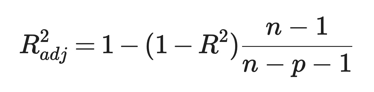
Adjusted R-squared formula

Here, p is the number of predictors, and higher values are better. The penalty is mild. A new predictor raises adjusted R-squared whenever the absolute value of its t-statistic is above 1, so it's the most lenient of the four criteria.

On the house data, adjusted R-squared keeps lot_size_sqft and rejects bedrooms by a margin in the fifth decimal place.

Same data, same forward search, different answers:

Variable selection based on different criteria

Stepwise Regression in Python and R

Both languages can run stepwise regression, but they do it in different ways. I'll use the same house price data from the example above in both.

Stepwise regression in Python

Python doesn't have a standard stepwise regression function.

Neither statsmodels nor scikit-learn has an equivalent of R's step() that selects predictors by AIC or p-values. So the most transparent option is to write the loop yourself on top of statsmodels. It's about 25 lines, and you can see every decision it makes.

To be clear, the forward_selection() function below is my own helper, not a statsmodels feature. statsmodels only fits the models and reports their .aic and .bic attributes.

First, generate the dataset and save it, so the R section can use the exact same rows:

import numpy as np
import pandas as pd
import statsmodels.formula.api as smf

rng = np.random.default_rng(42)
n = 200

square_feet = rng.normal(1800, 450, n).clip(700, 3500)
bedrooms = np.clip(np.round(square_feet / 600 + rng.normal(0, 0.6, n)), 1, 6)
age_years = rng.uniform(0, 60, n)
distance_km = rng.uniform(1, 30, n)
lot_size_sqft = rng.normal(6000, 1500, n).clip(2000, 12000)

# Bedrooms has no direct effect on price, lot size has a small one
price = (
    60000
    + 140 * square_feet
    - 1200 * age_years
    - 3500 * distance_km
    + 4 * lot_size_sqft
    + rng.normal(0, 45000, n)
)

house = pd.DataFrame({
    "square_feet": square_feet,
    "bedrooms": bedrooms,
    "age_years": age_years,
    "distance_km": distance_km,
    "lot_size_sqft": lot_size_sqft,
    "price": price,
})

house.to_csv("house_prices.csv", index=False)

Next, the selection loop. It starts from the intercept-only model, fits one model per remaining candidate, and keeps the addition with the lowest criterion value:

def forward_selection(data, target, candidates, criterion="aic"):
    selected = []
    remaining = list(candidates)

    # Score the intercept-only model first
    null_model = smf.ols(f"{target} ~ 1", data=data).fit()
    current_score = getattr(null_model, criterion)
    print(f"Start: {criterion.upper()} = {current_score:.1f}")

    while remaining:
        # Fit one model per remaining candidate
        scores = {}
        for candidate in remaining:
            formula = f"{target} ~ {' + '.join(selected + [candidate])}"
            scores[candidate] = getattr(smf.ols(formula, data=data).fit(), criterion)

        best = min(scores, key=scores.get)

        # Stop when the best addition doesn't lower the criterion
        if scores[best] >= current_score:
            print(f"Stop: adding {best} gives {scores[best]:.1f}")
            break

        selected.append(best)
        remaining.remove(best)
        current_score = scores[best]
        print(f"Add {best}: {criterion.upper()} = {current_score:.1f}")

    return selected


candidates = ["square_feet", "bedrooms", "age_years", "distance_km", "lot_size_sqft"]

aic_predictors = forward_selection(house, "price", candidates, criterion="aic")
print()
bic_predictors = forward_selection(house, "price", candidates, criterion="bic")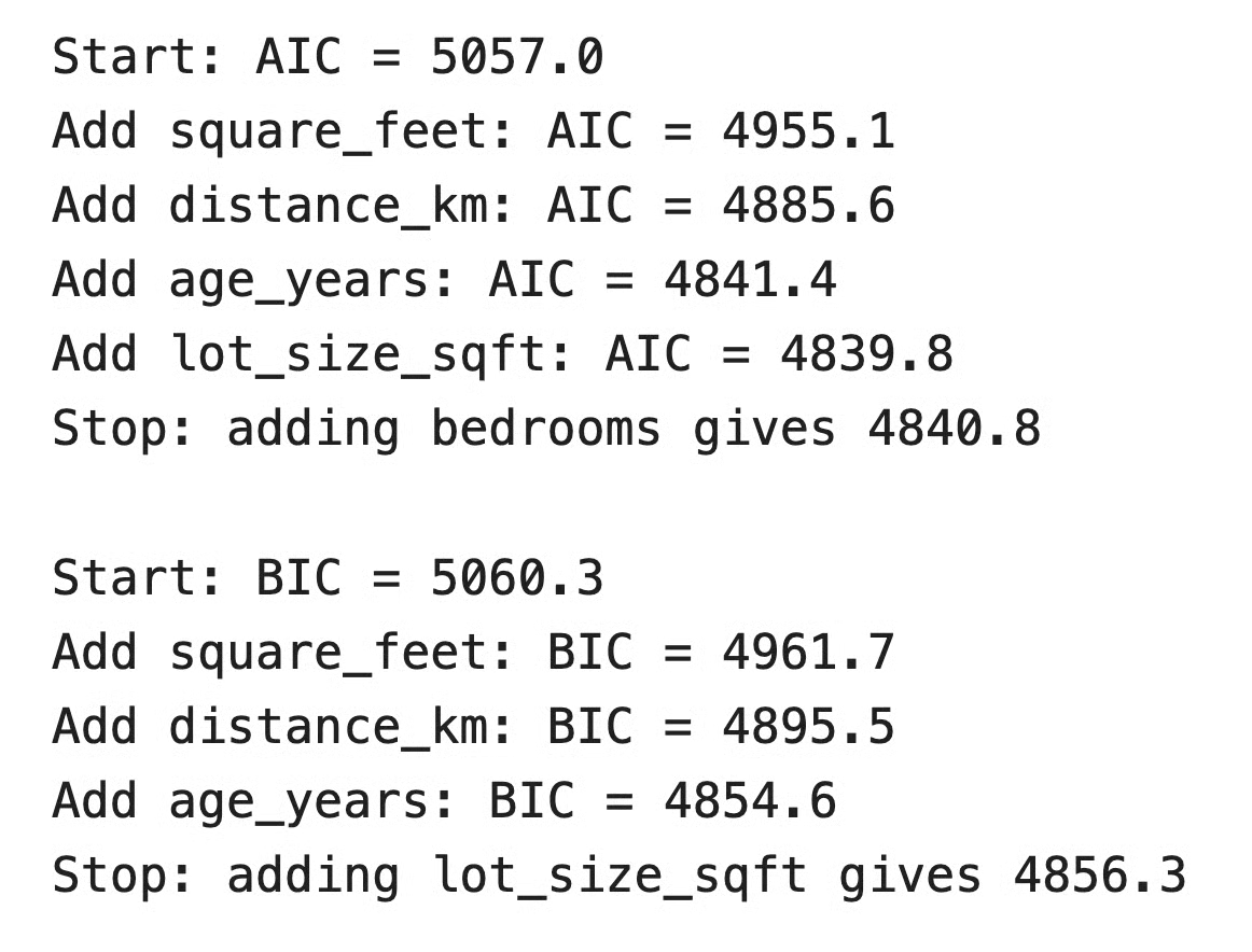

Forward selection in Python

These are the same AIC values from the example table. AIC ends with four predictors, and BIC stops at three because lot_size_sqft doesn't clear its bigger penalty.

If you'd rather use a package, scikit-learn has SequentialFeatureSelector. It runs forward or backward selection, but it scores each candidate with cross-validation instead of AIC or p-values:

from sklearn.feature_selection import SequentialFeatureSelector
from sklearn.linear_model import LinearRegression

X = house.drop(columns="price")
y = house["price"]

sfs = SequentialFeatureSelector(
    LinearRegression(),
    n_features_to_select="auto",
    tol=0.001,
    direction="forward",
    scoring="r2",
    cv=5,
)
sfs.fit(X, y)
print(list(X.columns[sfs.get_support()]))

Selected features in Python

With n_features_to_select="auto", the search stops when the cross-validated R-squared improves by less than tol. On this data, it ends with the same four predictors as AIC.

Stepwise regression in R

R has stepwise regression built in.

The step() function comes with base R's stats package, so there's nothing to install. You give it a starting model, a scope that defines the largest model it may consider, and a direction:

# Load the same data generated in the Python section
house <- read.csv("house_prices.csv")

# Intercept-only model and full model
null_model <- lm(price ~ 1, data = house)
full_model <- lm(
  price ~ square_feet + bedrooms + age_years + distance_km + lot_size_sqft,
  data = house
)

# Forward selection with AIC
aic_model <- step(null_model, scope = formula(full_model), direction = "forward")

# Forward selection with BIC
bic_model <- step(
  null_model,
  scope = formula(full_model),
  direction = "forward",
  k = log(nrow(house))
)

formula(aic_model)
formula(bic_model)

AIC and BIC formulas in R

The criterion step() minimizes is controlled by one argument - k.

It computes -2 log-likelihood + k * edf, where edf is the number of estimated coefficients. The default k = 2 gives you AIC. If you set k = log(n), you get BIC, but the printed trace still labels the values as "AIC", so don't let that confuse you.

For backward elimination, start from the full model:

backward_model <- step(full_model, direction = "backward")

On this data, it removes bedrooms and stops with the same four predictors as forward AIC. If you pass a scope and leave out direction, step() defaults to bidirectional selection.

Stepwise Regression vs Other Feature Selection Methods

Stepwise regression isn't the only way to choose predictors. Here's how it compares to three popular alternatives.

Stepwise regression vs. best subset selection

Stepwise regression is a greedy search. At each step, it makes the best single move and never looks back, unless you run it in both directions.

Best subset selection fits every possible combination of predictors and keeps the one with the best criterion value. With 5 predictors, that's 32 models. With 20, it's over a million, and with 40, it's over a trillion. Algorithms like branch-and-bound in R's leaps package can skip a lot of that work, but the cost still grows fast with the number of predictors.

On the house price data, best subset selection with AIC picks the same four predictors as forward selection. That won't always be the case, so keep that in mind.

Stepwise regression vs. Lasso regression

Stepwise regression makes yes-or-no decisions. A predictor is either in the model with its full least-squares coefficient, or out with a coefficient of zero.

Lasso regression fits all predictors at once and adds a penalty on the sum of absolute coefficient values. That penalty shrinks every coefficient toward zero and pushes the weakest ones all the way to zero, so selection and estimation happen in one step.

A small change in the data moves Lasso coefficients a little, while it can flip a stepwise decision from in to out. You choose the penalty strength with cross-validation, for example with LassoCV in scikit-learn or cv.glmnet() in R.

The shrunken coefficients are biased toward zero on purpose. It's a trade you make for more stable estimates and better out-of-sample predictions.

Stepwise regression vs. recursive feature elimination

Recursive feature elimination, or RFE, looks like backward elimination. You fit a model on all features, remove the weakest ones, refit, and repeat.

The difference is what "weakest" means. Backward elimination uses a statistical criterion like AIC or a p-value. RFE uses the model's own importance scores, such as coefficient magnitudes or tree-based feature importances.

That makes RFE a machine learning tool first. It works with any model that has feature importance, including random forests and support vector machines, and you usually pair it with cross-validation through RFECV in scikit-learn. You get a feature set that predicts well, but no likelihood-based criterion and no p-values.

Problems with Stepwise Regression

Stepwise regression is easy to run and explain. That's exactly why its problems are easy to miss.

Statisticians have criticized the method for decades - Frank Harrell's Regression Modeling Strategies and Whittingham et al. (2006) in the Journal of Animal Ecology are two well-known examples. In a 2018 paper in the Journal of Big Data, Gary Smith argues that stepwise regression is less effective the larger the number of potential explanatory variables, so it doesn't solve the problem of too many predictors.

Unstable variable selection

Small changes in the data can change which predictors you get.

If you remove a couple of rows or collect a new sample from the same population, stepwise can return a different model. Predictors near the selection threshold are the most fragile. A predictor with a real but small effect, like lot_size_sqft in the house price example, can enter in one sample and stay out in the next. A predictor with no effect, like bedrooms, can sneak in when the sample happens to favor it.

This matters because you only ever see one sample. The model stepwise gives you is one of a range of possible models, and the output doesn't tell you how wide that range is.

Biased coefficient estimates

Stepwise uses the same data to choose predictors and to estimate their coefficients.

A weak predictor makes it into the model mostly in samples where its effect happens to look stronger than it is. In samples where it looks weaker, it gets left out. So the coefficients you see after selection are too large on average.

In plain English, stepwise regression reports the winners, and winners look better than they are.

Misleading p-values and confidence intervals

The p-values in a regression summary assume you chose the model before you looked at the data.

Stepwise does the opposite. It runs a batch of tests, keeps the predictors that pass, and then reports p-values as if those predictors were the only ones you ever tested. So the p-values come out too small and the confidence intervals too narrow.

The problem is worse when a lot of candidates have no effect. David Freedman showed this in a 1983 paper in The American Statistician - when he screened pure noise predictors and refit the model, the result looked statistically significant even though there was nothing to find. Smith makes the same point: nuisance variables may be coincidentally significant, while real ones can miss the threshold.

If you report those p-values as evidence, you may be reporting noise.

Overfitting

Overfitting is the prediction side of the same problem.

Every candidate predictor gives stepwise another chance to fit a pattern that exists only in your sample. The selected model looks good on the data it was built on, but those patterns don't repeat in new data. As a result, the model may fit the data well in-sample, but do poorly out-of-sample.

And the more candidate predictors you give it, the more chances it gets to find patterns that aren't there.

Correlated predictors

When two predictors have similar information, stepwise has to choose between them, and small differences in the sample decide the choice.

square_feet and bedrooms in the house data are a mild example - once square_feet is in the model, bedrooms adds almost nothing. With stronger correlation, the choice becomes close to random. One sample keeps variable A, the next keeps variable B, and each model tells a different story about what drives the outcome.

Neither story is reliable. Stepwise can't tell you that two predictors are interchangeable so it just picks one.

Greedy search

Stepwise makes one decision at a time, and each decision depends on the ones before it.

That means it can miss the best model. Let's say two predictors are useless on their own but strong together, which can happen when each one corrects for noise in the other. Forward selection will never add either one, because neither improves the model in a single step.

Backward elimination and bidirectional selection reduce this risk, but they don't remove it. None of the three checks all combinations, so none of them can promise the best model for the chosen criterion.

When Should You Use Stepwise Regression?

Stepwise regression is a tool with a narrow job.

It's a good choice for:

1. Exploratory analysis: It gives you a quick first look at which predictors might matter, as long as you treat the result as a hypothesis
2. Teaching variable selection: The step-by-step trace makes the idea of model selection easy to see, including its problems
3. Reducing a candidate set: It can narrow down a long list of predictors before you look at them more closely, if you check the result for stability
4. Automated baseline models: It gives you a quick reference model to compare more careful models against

It's the wrong choice for confirmatory inference and causal analysis.

If your goal is to test whether a predictor has an effect, the p-values after stepwise selection can't answer that question. And if your goal is causal, the right set of variables comes from how the data was generated, and not from which variables lower AIC. Stepwise has no idea which variable causes which.

For prediction, you have better options. Regularization methods like Lasso and elastic net are more stable, and cross-validated feature selection judges models on data they didn't see.

Best Practices for Stepwise Regression

If you decide to use stepwise regression, these steps can make the results more honest:

1. Start with plausible predictors: Only include candidates you can justify with domain knowledge, since every extra candidate gives the algorithm another chance to pick noise
2. Choose the criterion on purpose: AIC leans toward prediction, BIC toward smaller models, and p-value thresholds are conventions, so pick the one that aligns with your goal and decide before you run anything
3. Don't take selected p-values at face value: Treat them as descriptive, not as evidence, because the selection already used the data they're based on
4. Validate on unseen data: Evaluate the final model on a holdout set or with cross-validation of the whole procedure, not just the final model
5. Check multicollinearity: Look at correlations and variance inflation factors among the candidates, so you know which choices might be close to random
6. Test stability: Rerun the selection on bootstrap samples and report how often each predictor gets selected
7. Compare against other models: Fit a Lasso model and a model built from domain knowledge, and see whether stepwise does any better on held-out data
8. Report the procedure: Write down the candidate set, the direction, the criterion, and the thresholds, so others can reproduce and judge the result

Conclusion

Stepwise regression automates predictor selection. It adds or removes one variable at a time and stops when no change improves the model by your chosen criterion.

Forward selection starts empty and only adds. Backward elimination starts with the full model and only removes. Bidirectional selection does both, so it can undo an earlier decision.

But the simplicity means the selected predictors can change from sample to sample, the model can fit noise, and the p-values and confidence intervals after selection aren't reliable. That's something to keep in mind. So treat stepwise regression as one model-selection technique. It's not the default way to build a regression model.

If you want to go further, read up on feature selection in general, see how AIC and BIC compare models, and try Lasso regression as a first step into regularization.