t Statistic Explained: Formula, Interpretation, and Examples

The t statistic shows whether an observed difference is meaningful or likely due to random variation.

Differences appear in almost every dataset. The key question is whether the result reflects a real effect. The t statistic answers that by comparing the size of the difference to the uncertainty in the data.

This is why it is widely used in hypothesis testing and regression. It helps you judge whether a result is statistically significant and worth taking seriously.

In this guide, you will learn what the t statistic means, how to calculate it, how to interpret it, and how to apply it in common testing scenarios.

What is the t-statistic in Statistics?

The t statistic measures how far a result is from a reference value after adjusting for variability in the data.

In simple terms, it is the difference scaled by uncertainty. This converts a raw gap into a standardized value you can evaluate.

Consider a class with an average score of 78 compared to a benchmark of 75. The difference is 3 points. That number alone does not tell you much. If the scores are tightly grouped, the gap may be meaningful. If the scores vary widely, the same gap may not matter.

The t statistic combines both pieces into one value. It shows whether the observed difference is large relative to the variation in the data.

This is important because the same difference can lead to different conclusions depending on how stable the data is. The t statistic puts the result in context so you can judge its significance.

You will see it used in common scenarios:

• One sample t test checks if a sample mean differs from a known value
• Two sample t test compares the means of two groups
• Paired t test compares the same group before and after a change
• Regression analysis tests whether a coefficient differs from zero

Across all of these cases, the logic stays the same: measure the distance from a reference point, adjust for variability, and evaluate whether the result is meaningful.

t Statistic Formula and How It Is Calculated

The t-statistic follows a simple structure. It compares what you observed with what you expected, then scales that difference by uncertainty.

In this formula:

• The estimate is your sample result

• The hypothesized value is what you are testing against

• standard error measures how much your estimate can vary due to randomness

So the t-statistic tells you how many standard errors your result is away from the value you are testing.

One-sample t statistic

You use this when you compare one sample average to a known value.

Here: 

• x is the sample mean

• μ0 is the hypothesized value

• s is the sample standard deviation

• n is the sample size

The denominator s/n​ is the standard error of the mean.

Two-sample t statistic (independent samples)

This test compares the means of two separate groups. The structure stays consistent:

• Numerator: difference between the two sample means
• Denominator: standard error of that difference

But here is a slight change: When you calculate the standard error, you need to decide how to treat the variability in both groups.

There are two common approaches.

1. Unequal variances

Use this when the groups have different levels of spread, which is common in real data:

• Each group keeps its own variance
• Both variances are combined when calculating the standard error

2. Equal variances 

Use this when both groups show similar variability:

• Variances are combined into a single pooled estimate
• The calculation becomes simpler

Regression coefficient t statistic

In regression, each coefficient has its own t statistic.

• Numerator: estimated coefficient
• Denominator: standard error of that coefficient

This shows whether a predictor has a meaningful relationship with the outcome variable.

A quick numeric example

Consider a one-sample case:

• Sample mean = 78
• Hypothesized value = 75
• Sample standard deviation = 10
• Sample size = 25

Step 1: Compute the standard error

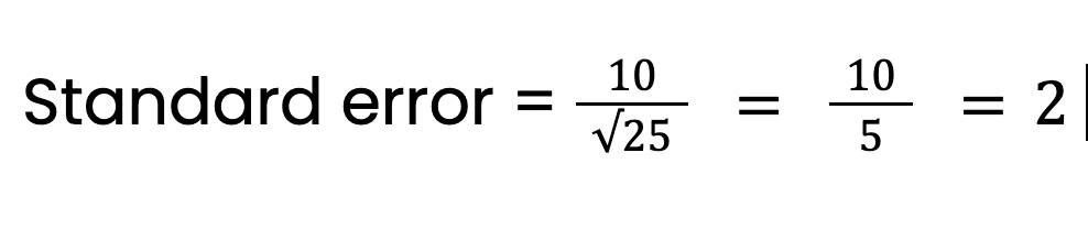
Step 2: Find the difference

Difference = 78 − 75 = 3

Step 3: Compute the t statistic

T = 3/2 = 1.5

The sample mean is 1.5 standard errors above the reference value. This value is used in the next step to assess statistical significance.

The t Distribution and Degrees of Freedom

The t statistic only becomes useful when you compare it to a reference distribution. That reference is the t distribution.

It shows what t-values look like when there is no real effect. Once you calculate a t value, you check where it falls on this distribution. Values far from the center are less likely to occur by chance. Values near the center are more consistent with random variation.

What degrees of freedom mean

Degrees of freedom control the shape of the t distribution. They reflect how much reliable information your data provides: more data leads to more stable estimates and less data increases uncertainty.

Some of its common formulas are:

• One-sample t test: degrees of freedom = n − 1
• Two-sample t test: degrees of freedom = n₁ + n₂ − 2
• Regression: degrees of freedom = n − k − 1, where k is the number of predictors

How sample size affects the distribution

With small samples, variability is harder to estimate. This makes extreme t-values more likely, so the t distribution is wider.

This leads to two outcomes:

• Larger t values are required to show significance
• Results are harder to classify as meaningful

As the sample size increases, estimates become more stable. The t distribution narrows and starts to match the normal distribution. With large samples, the difference between the two is minimal.

How to Interpret the t Statistic

A larger t-statistic means stronger evidence against the null hypothesis. A smaller t-statistic means the result may be due to random variation.

That is the core idea. Now let’s make it practical.

What does the size of t tell you

Focus on how far the value is from 0.

• t close to 0 > little to no difference
• larger t > stronger difference
• very large t > strong evidence against the null

The sign only shows direction.

• positive > above the expected value
• negative > below the expected value

For interpretation, the magnitude is more important than the sign.

How to get the p-value

After calculating the t statistic, compare it to the t distribution. This gives the p value, which shows how likely your result is under the null hypothesis.

• small p value > result is unlikely under the null, stronger evidence against it
• large p value > result is likely under the null, weak evidence

The t statistic gives the distance. The p value shows how unusual that distance is.

One-tailed vs. two-tailed tests

The choice depends on your hypothesis:

• Two-tailed test checks for any difference, higher or lower
• One-tailed test checks for a difference in a specific direction

Two-tailed tests are more common. One-tailed tests are used only when the direction is defined before analysis.

Statistical significance vs. practical importance

A result can be statistically significant and still not useful. This happens often with large datasets.

• With large samples, even small differences can appear statistically significant
• With small samples, meaningful differences may not appear significant

So do not rely on the p-value alone. Look at the size of the effect and ask if it matters in real decisions.

t Statistic in Hypothesis Testing

The t statistic is used to test whether a result is meaningfully different from a reference value, often zero. That reference represents no effect or no difference. 

It answers a single question: is the observed result large enough to treat as real rather than random variation.

Testing a population mean

Use this when comparing a sample mean to a known or assumed value.

Suppose the average time on a page is expected to be 5 minutes and your sample shows 6 minutes. The t statistic evaluates whether this 1 minute gap is meaningful.

• small t value means difference is likely due to chance
• large t value means difference is likely real

This forms the basis for rejecting or not rejecting the null hypothesis.

Comparing two means

Use this to compare two independent groups.

Take conversion rates for two landing pages as an example:

• Group A: old design
• Group B: new design

A higher average in one group is not enough on its own. The t statistic checks whether the gap between the two averages is statistically significant.

Larger absolute t value means stronger evidence that the difference is real. 

Paired samples testing

Use this when the same group is measured twice.

Suppose you have user engagement before and after a feature update. Each observation is linked. You work with the differences within each pair rather than comparing separate groups.

The t statistic tests whether the average change across all pairs differs from zero. This shows whether the change had a meaningful effect.

Testing regression coefficients

In regression, each coefficient has its own t statistic. Each coefficient represents the relationship between a predictor and the outcome.

Suppose a coefficient may represent the effect of email frequency on conversions. The t statistic tests whether that coefficient differs from zero.

• value close to zero means little or no effect
• value far from zero means likely meaningful effect

This helps identify which variables contribute to the model.

T Statistic Table

A t table helps you decide whether your result is statistically significant. It provides critical values based on:

• degrees of freedom
• chosen significance level (such as 0.05) 

How to use the t table

Follow these steps:

1. Calculate your t statistic
2. Find your degrees of freedom
3. Choose your significance level
4. Look up the critical value in the table

Now compare your result with the critical value:

• If your t value is larger than the table value, it means statistically significant
• If it is smaller, it’s not statistically significant

Here’s how to read this table. 

Let’s say:

• Your t-statistic = 2.3
• Degrees of freedom = 10
• Significance level = 0.05

From the table:

• Critical value = 2.23

Now compare:

• Your t = 2.3
• Table value = 2.23

Since 2.3 is greater than 2.23, the result is statistically significant.

t Statistic vs. z Statistic: What’s the Difference?

The key difference is simple:

• Use the t statistic when the population standard deviation is unknown
• Use the z statistic when it is known

Learn more about the difference between t statistics and z statistics in our guide. 

When to use the t statistic

Use the t statistic when working with sample data and you do not know the population standard deviation.

This is the common case. You estimate variability using the sample standard deviation, which introduces uncertainty. The t statistic adjusts for that uncertainty, making it suitable for smaller datasets.

Let’s say you collect data from 25 users to estimate the average session time. Since the true population variability is unknown, you use the t statistic.

When to use the z statistic

Use the z statistic when the population standard deviation is known.

This is less common but can apply in controlled environments or when you have stable historical data. It is also used with very large samples, where the sample standard deviation closely matches the population value.

If a company has long-term data and knows the exact standard deviation of a metric, it can use the z statistic for testing.

Why sample size matters

Sample size affects how much uncertainty exists in your estimates.

• small samples: higher uncertainty so t statistic is more appropriate
• large samples: lower uncertainty so z statistic becomes reasonable

The t distribution accounts for this by being wider for small samples, which leads to more conservative results.

How t and z become similar

As sample size increases, the difference between the two methods becomes minimal. With large datasets, both approaches produce nearly identical results. This is why the z statistic is often used as an approximation in large-scale analysis.

t Statistic vs. t Test: What’s the Difference?

The t statistic is a single value, and the t test is the full decision process. Let’s understand both:

What is the t statistic?

We covered this a lot so far, but let me reiterate: The t statistic is calculated from your sample data. It shows how far your result is from the null hypothesis value, usually zero.

It gives you the size of the difference relative to the variability in the data. On its own, it does not tell you whether the result is significant.

What is the t-test?

The t-test is a specific way of doing a hypothesis test.

It includes:

• defining the null and alternative hypotheses
• calculating the t statistic (above)
• finding the p value or critical value
• making a decision based on the result

This process determines whether the observed difference is statistically significant.

How they work together

The t statistic is one step within the t test.

You calculate the t value first. Then you use it to get a p value or compare it with a critical value. That final step allows you to decide whether to reject the null hypothesis.

Common Mistakes When Using the t Statistic

Most errors come from interpretation, not calculation. The t statistic is easy to compute but easy to misuse if key details are ignored.

Judging the t value without context

A large t value on its own does not tell you much. Its meaning depends on sample size and variability.

What to do:

• interpret the t value with the p value
• consider the sample size
• check how much variation exists in the data

Ignoring key assumptions

The t statistic relies on a few conditions. If they are not met, results may be unreliable. Main assumptions are:

• data is roughly normal, especially for small samples
• observations are independent

What to do:

• check the data distribution
• use plots or summary statistics to identify issues
• use alternative methods if assumptions are violated

Mixing up one-tailed and two-tailed tests

Choosing the wrong test changes the conclusion. One-tailed test checks one direction and two-tailed test checks both directions

What to do:

• decide the test type before analysis
• use two-tailed tests by default unless a specific direction is required

Running multiple t-tests instead of ANOVA

Comparing more than two groups with multiple t tests increases the risk of false positives.

Here's what to do: Use ANOVA for three or more groups. Then, follow up with post hoc tests if needed

Relying only on p-values

A small p-value shows statistical significance, not practical importance. Make sure you check the effect size and assess whether the result matters in real decisions.

Conclusion

Differences appear in all datasets. The challenge is knowing whether they reflect a real effect or random variation. The t statistic addresses this by scaling the difference based on uncertainty.

Without the t statistic, you only see differences. With it, you can evaluate whether those differences are worth acting on.