What Is Flow Matching? A Guide to Generative AI Models

Have you seen the term "flow matching" next to every new image and video model, and have no idea what it stands for?

Most explanations either go straight into differential equations or present it as "diffusion, but better." Neither tells you what the model learns. Stable Diffusion 3 and Flux both run on flow matching, and they generate images in a couple of steps where classical diffusion needs dozens.

This is the general idea: instead of learning individual examples, the model learns a velocity field that tells any sample which direction and how fast to move. Once you understand that, the training process, the math behind it, and its relationship to diffusion will all make sense.

In this article, I'll walk you through the intuition behind flow matching, how it's trained, the math (while keeping it light), and how it compares to diffusion models.

If you're new to AI for image data, read our Top 10 Vision Language Models in 2026 to discover the current state-of-the-art models for visual reasoning, image analysis, and computer vision.

What Is Flow Matching?

Flow matching is a training objective, not a model architecture.

That distinction is important because you can pair it with a transformer or almost any other network - what makes it flow matching is what the network gets trained to predict, not what the network looks like.

And what it's trained to predict is a time-dependent vector field. In plain English, that's a function that tells you which direction and how fast a sample should move at each point along its path from the source distribution to the target distribution. When you train it to train continuous normalizing flows this way, you get a model that turns a simple distribution into a complex one, step by step.

I like to break the intuition in four ideas:

• Start simple: Begin with a distribution you can sample from easily, such as Gaussian noise
• Define paths: Connect each noise sample to a target data point along a smooth path
• Learn the motion: Train a network to predict how a sample should move along that path, at every point in time
• Follow the flow: Once trained, start from noise and follow the learned vector field to produce new samples

If you're more of a visual type, imagine a cloud of scattered particles with no order to them. Flow matching teaches each particle exactly which direction to move and how fast, so the whole cloud settles into a structured pattern over time (the shape of your target distribution).

When you run this on an image dataset, "structured pattern" means a coherent photo instead of random noise.

How Flow Matching Works

Training and generation are two separate phases here, and confusion often starts when people think they're the same.

During training:

• Sample a data point: Choose a point from your training set - the target your samples move toward
• Sample noise: Pick a point from a simple source distribution, usually Gaussian noise
• Pick a time: Choose a random t between 0 and 1
• Build an intermediate point: Combine the data point and the noise sample according to t, based on a probability path that connects the two
• Get the target velocity: Work out the direction and speed that intermediate point should have at time t, based on the path you chose
• Train the network: Teach it to predict that velocity, given the intermediate point and the time

Generation doesn't need the data point.

You start from noise and integrate the learned vector field forward in time, one small step at a time, until you get to a sample from the data distribution.

And that's the idea - you predict velocity during training, and follow it during generation.

Understanding Vector Fields and Probability Paths

There are two ideas that do most of the work behind the flow matching objective - vector fields and probability paths. Once you understand them, the loss function in the next section will make sense.

Vector fields

A vector field is what the network predicts. At any point in space and at any moment in time, it gives you a direction and a speed - the way a sample at that point should move to get closer to the data distribution.

For example, imagine standing in a river. Wherever you're standing, the current pushes you a certain way, and how hard and in which direction depends on your exact position and the moment in time. A vector field does the same thing for your samples - it assigns a direction and a speed to every point in space, at every point in time.

Probability paths

A probability path is the sequence of distributions a sample moves through on its way from noise to data. At t = 0, you're sampling from the source distribution, usually Gaussian noise. At t = 1, you're sampling from the target data distribution. Everything between those two points is an intermediate distribution, and the probability path describes how one turns into the next.

The vector field and the probability path are directly connected because the vector field moves samples along the probability path, from one intermediate distribution to the next, until they reach the data distribution.

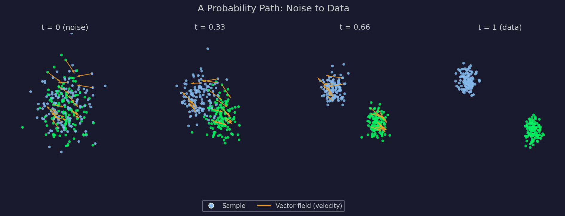
A probability path diagram

The Flow Matching Objective

The flow matching objective turns vector fields and probability paths into a single regression loss.

Every training step compares two velocities. The first is the target velocity - the direction and speed a sample should move at that point along the chosen probability path. The second is the model-predicted velocity - the network's own guess for that same direction and speed, based on the current sample and time. Training makes those two match as closely as possible.

Here's the loss function:

Flow matching loss function

Here's what each term means:

• v_θ(x_t, t): The model's predicted velocity at point x_t and time t

• u_t(x_t): The target velocity at that same point and time, based on the chosen probability path

• 𝔼[...]: An average over many random values of t and x_t

• ‖ · ‖^2: The squared difference between the two velocities - plain mean squared error

The full derivation is beside the point here. What matters is that the network predicts a single vector at a single point and time, and you compare it to a known target. That's it!

Conditional Flow Matching

The marginal probability path connecting the full noise distribution to the full data distribution isn't something you can write down directly.

Computing the target velocity at a given point means accounting for every data sample that could have produced it - an integral over your entire dataset, not something anyone computes at every training step.

Conditional flow matching solves this by conditioning on individual samples instead of the full path. Rather than computing the vector field for the entire marginal path, you choose a single data point and a single noise point, then construct a probability path just for that pair. When you make that conditional path simple, for example with a straight line between the two points works, the target velocity has a closed-form expression you can directly compute.

Training the network on these simple, per-pair conditional velocities, averaged across enough pairs, gets you the same vector field you'd get from the intractable marginal objective. You never directly compute the marginal path - instead, you approximate it indirectly, one easy conditional path at a time.

This conditional version is the one almost everyone actually trains. The marginal formulation makes the math work, but the conditional formulation is what works in practice.

Flow Matching vs Diffusion Models

Diffusion and flow matching keep getting compared for a good reason - most of the "diffusion models" you already know now run on a flow matching objective. That doesn't mean flow matching replaced diffusion. It means diffusion turned out to be one specific case inside a bigger framework, and flow matching is the general version of it.

Let me start with what each network predicts. A diffusion model predicts noise. Given a noisy sample and a time step, it predicts the noise that was mixed in, then removes it, one step at a time. Flow matching predicts a velocity instead. Given a sample and a time step, it predicts which direction and how fast that sample should move toward the data distribution.

The probability path is where the two differ the most.

Diffusion models fix one specific noising process up front, usually adding Gaussian noise on a fixed schedule, and everything else follows from that single choice. In flow matching, you choose any path connecting noise to data, and the objective works the same way no matter which one you pick. A diffusion-style Gaussian path is one option. A straight line between noise and data is another, and it turns out to matter a lot for how fast you can sample.

These two predictions aren't as different as they look.

A diffusion model's noise prediction and a flow matching model's velocity prediction are two views of the same underlying object, connected through the score of the distribution at each point in time. Where they differ is in how they generate. Diffusion sampling is stochastic by default, meaning each denoising step adds a bit of randomness back in (though deterministic variants like DDIM exist). Flow matching works the other way - its natural formulation is a deterministic ODE, so the same starting noise produces the same output every time, and stochastic versions exist on that side too.

Sampling in both cases means solving a differential equation step by step, moving from noise toward data.

Diffusion models tend to need dozens of steps unless you include fast samplers or distillation. Flow matching, especially when trained on straight-line paths, tends to need far fewer steps without any of that - a straight path has a constant velocity, which is much easier for a solver to follow accurately than a curved one.

The path itself is where flow matching gets ahead.

Diffusion models are limited to whatever noising process they were derived from. Flow matching treats the path as a design choice, and different choices come with different trade-offs.

Flow matching compared to diffusion models

Flow Matching vs. Related Generative Methods

Diffusion isn't the only method that gets compared to flow matching. There are three more you should know about

Flow matching vs. continuous normalizing flows

Continuous normalizing flows came first, and flow matching grew directly out of the issues with training them.

A continuous normalizing flow is the kind of model flow matching produces - a network that defines a continuous transformation between distributions through an ODE. Training one the original way meant solving that ODE forward and computing an exact likelihood at every step, which means tracking how the transformation changes probability density along the way. That computation is expensive, and it only gets worse as the network grows.

Flow matching avoids all of that. It regresses directly on a known target velocity instead of solving the ODE and computing likelihoods during training. There is no simulation required. You still end up with a continuous normalizing flow, you just don't pay the earlier training cost to get there.

Flow matching vs. score matching

Score matching trains a network to predict the score - the gradient of the log probability density - at each noise level. That's the objective behind the diffusion models you already know.

Flow matching trains a network to predict a velocity instead. The two objects are mathematically related, meaning that under certain path choices, you can convert one into the other. But they represent different things. The score describes the shape of the probability distribution at a fixed point in time. The velocity describes how a sample should move as time changes.

Score matching asks about geometry. Flow matching asks about motion.

Flow matching vs. rectified flow

Rectified flow is a specific choice inside flow matching.

Flow matching lets you pick any probability path connecting noise to data. Rectified flow picks one - straight lines, and then goes a step further with an iterative procedure called "reflow" that straightens the paths a trained model already learned, so a second-round model needs even fewer integration steps at generation time.

That's why the two terms show up side by side in the same papers. Stable Diffusion 3 and Flux both use flow matching with something close to a rectified-flow path choice. But treating flow matching and rectified flow as interchangeable misses the point. Flow matching is the framework. Rectified flow is one path you can choose inside it.

Flow Matching in Modern Generative AI

Flow matching is now running inside some of the biggest generative systems in production.

• Image generation is where flow matching first showed up at scale. Stable Diffusion 3 moved from the older DDPM-style formulation to flow matching, and Flux, from Black Forest Labs, builds on a similar rectified-flow approach. Both get faster and higher-quality sampling out of the straight-path idea covered above.
• Video generation is where the freedom to choose your own path makes sense, because video is expensive to sample even one frame of, let alone dozens of them at every denoising step. Meta's Movie Gen Video, a 30-billion-parameter model, replaces the usual diffusion U-Net with a Transformer trained under a flow matching objective. A couple of large video generators released since then use the same approach inside the latent space of a pretrained video encoder, for the same reason - fewer sampling steps mean real savings at that scale.
• Audio and speech generation benefits from flow matching too. Meta's Voicebox used it for multilingual speech generation back in 2023, and Movie Gen's audio component generates soundtracks and sound effects the same way, synced to the video it accompanies. Open TTS systems like F5-TTS build directly on flow matching with a diffusion transformer, producing natural speech without a separate duration model or phoneme aligner.
• Multimodal generation shows up less as a separate technique and more as the payoff of using one objective everywhere. Movie Gen itself is framed as a cast of media foundation models - video, audio, personalization, and editing, all trained under the same flow matching objective.

All of this is because a regression loss is simple to implement and simple to scale. And because the path is a design choice, teams building billion-parameter systems can pick one that needs fewer sampling steps, and that matters when every step costs compute at that scale.

A Simple Flow Matching Example

Everything so far was conceptual. I'll now walk you through the same idea running on an actual 2D dataset, small enough to see every step of it.

The noise distribution is a standard 2D Gaussian, centered at the origin. The target distribution is three Gaussian clusters arranged in a triangle - simple enough for a small network to learn quickly, but structured enough that you can actually tell whether it got it right.

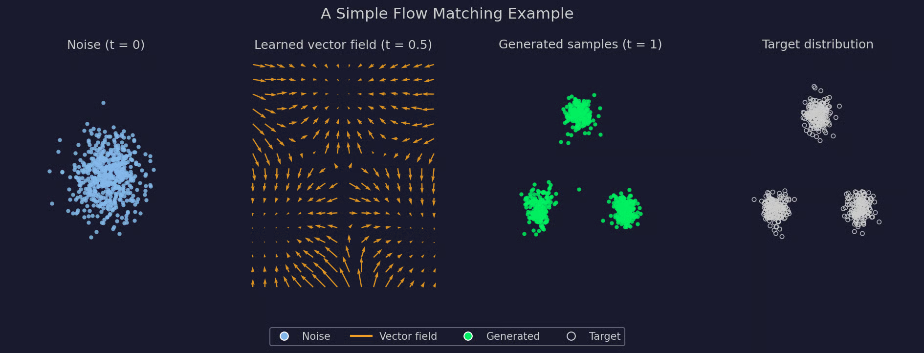
Simple flow matching example

The first panel is where every sample starts - scattered noise with no structure to it. The second panel is the vector field itself, evaluated on a grid at the midpoint of training. Notice how the arrows already point toward one of the three clusters, well before any sample gets there. The third panel shows what happens when you start from fresh noise and follow that field all the way to t = 1 - three clusters emerge, matching the fourth panel almost perfectly.

None of this involved anything the earlier sections didn't already cover - a source distribution, a target distribution, a learned vector field, and an ODE solver connecting the three. Onto the code.

Flow Matching in Python

Here's a small PyTorch implementation of the same example, using the same noise source and three-cluster target.

Start with the two distributions and how you sample from them:

import torch
import torch.nn as nn

torch.manual_seed(0)

# Three Gaussian clusters as the target ("data") distribution
centers = torch.tensor([[0.0, 3.0], [-2.6, -1.6], [2.6, -1.6]])

def sample_target(n):
    idx = torch.randint(0, 3, (n,))
    return centers[idx] + 0.4 * torch.randn(n, 2)

def sample_source(n):
return torch.randn(n, 2)

The network itself takes a point and a time step, and predicts a velocity:

class VelocityNet(nn.Module):
    def __init__(self, hidden=64):
        super().__init__()
        self.net = nn.Sequential(
            nn.Linear(3, hidden), nn.ReLU(),
            nn.Linear(hidden, hidden), nn.ReLU(),
            nn.Linear(hidden, 2),
        )

def forward(self, x, t):
    return self.net(torch.cat([x, t], dim=1))

Training samples a batch of source points, target points, and time steps on every step, then interpolates between the first two and regresses onto the resulting velocity:

model = VelocityNet()
optimizer = torch.optim.Adam(model.parameters(), lr=1e-3)

for step in range(3000):
    # source (noise) points
    x0 = sample_source(256) 
    # target (data) points
    x1 = sample_target(256) 
    # random time steps
    t = torch.rand(256, 1) 

    # interpolate along a straight-line path
    xt = (1 - t) * x0 + t * x1 
    # target velocity for that path
    target_v = x1 - x0 

    pred_v = model(xt, t)
    loss = ((pred_v - target_v) ** 2).mean()

    optimizer.zero_grad()
    loss.backward()
    optimizer.step()

Generation solves the learned ODE with plain Euler integration. You just need a loop that takes small steps from t = 0 to t = 1:

@torch.no_grad()
def generate(model, n_samples, n_steps=100):
    x = sample_source(n_samples)
    dt = 1.0 / n_steps
    for i in range(n_steps):
        t = torch.full((n_samples, 1), i * dt)
        x = x + model(x, t) * dt 
    return x

samples = generate(model, n_samples=600)
`

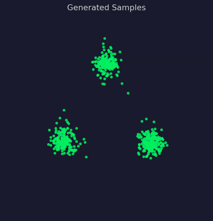
Generated samples visualization

And that's the entire pipeline! Sample, interpolate, regress, integrate. Nothing here changes if you go with a bigger network, a different path, or a higher-dimensional dataset - only the scale does.

Advantages and Limitations of Flow Matching

None of this makes flow matching a universal upgrade over diffusion. It's a trade-off, the same as any other design choice.

Here's where it's a good option and where it isn't.

Advantages

• Direct regression objective: There's no score estimation, no likelihood bounds, and no adversarial loss to balance - just a comparison between a predicted velocity and a known target
• Choice of probability path: You're not limited to one noising process; a straight-line path, a diffusion-style path, or a custom one all fit inside the same objective
• A natural fit for continuous-time models: Flow matching trains continuous normalizing flows without the expensive likelihood computation those models used to require
• Fewer sampling steps: Straighter paths mean an ODE solver needs fewer steps to stay accurate, which shows up as faster generation in practice
• Works across data types: The same objective trains image, video, audio, and multimodal models - none of the math changes with the modality

Limitations

• ODE integration can be expensive: Every sampling step still means a forward pass through the network, and that adds up at video or audio scale
• Quality depends on the path and the network: A poorly chosen probability path or an undertrained network still produces bad samples, straight-line paths included
• The math has a learning curve: Probability paths, vector fields, and continuous-time formulations take more background than a plain denoising picture
• Large models still cost what large models cost: Flow matching lowers the per-step cost of a system like Movie Gen or Flux, but training and running billion-parameter networks stays demanding either way

Conclusion

Flow matching teaches a model how samples should move from a simple distribution toward the data distribution. Everything else I described in this article exists to make that one idea trainable.

Two ideas do most of the work here. A probability path connects noise to data through a sequence of intermediate distributions. A vector field describes how a sample should move at any point along that path, at any moment in time. The network learns that vector field, its velocity, and generation is just following the resulting flow from noise to data.

None of this stands apart from what came before it. Flow matching is how modern systems train continuous normalizing flows without the old likelihood computation, and diffusion models turn out to be one specific case of it.

If diffusion models, normalizing flows, or generative AI more broadly interest you, that's exactly where to go next:

• Building a Diffuser Model From Scratch with PyTorch
• Introduction to Foundation Models
• Generative AI Concepts