Covariance vs. Correlation: What's the Difference?

In data analytics, we are forever trying to understand how variables relate to one another. You have probably encountered two statistical measures commonly used for this purpose: covariance and correlation. These measures sound similar and are often confused with each other. But what is the difference between them, and how should they be used?

Both describe how variables move together. However, despite their similarities, covariance and correlation answer slightly different questions and thus serve different roles in data workflows. Covariance captures the raw joint variability between features, while correlation standardizes that relationship so it can be compared more easily.

Let's explore how this subtle difference affects which measure we use in different circumstances.

What Is Covariance?

Covariance measures how two variables move together. It tells us whether increases in one variable tend to coincide with increases or decreases in another. There are three types of covariance:

• Positive covariance: When one variable increases as the other increases.
• Negative covariance: When one variable increases while the other decreases.
• Near-zero covariance: When there is no consistent directional relationship.

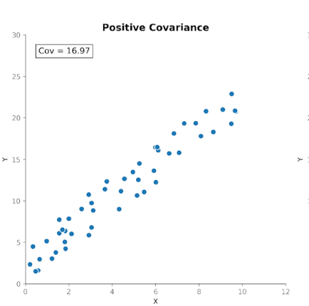
This makes covariance useful for detecting how variables move with respect to one another.

However, while the direction of the relationship is useful, interpreting the magnitude of the covariance is not so straightforward. The magnitude depends on the units of measurement as well as the scale of the variables. Converting units, for example, from centimeters to meters, can dramatically change the covariance magnitude without affecting the underlying relationship.

For this reason, covariance is more often used as an internal computational building block than as a standalone summary statistic.

What Is Correlation?

Correlation measures the strength, as well as the direction, of the relationship between two variables. It builds on covariance by standardizing the magnitude so that units no longer influence it.

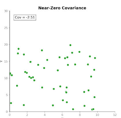
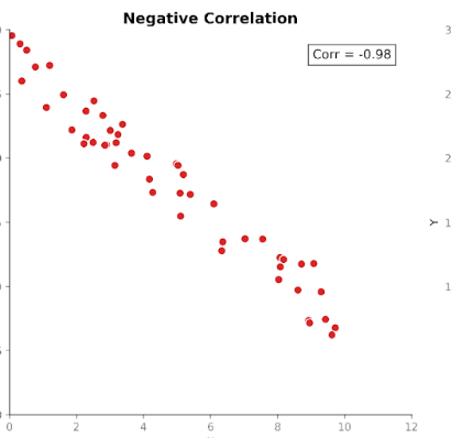
Correlation values fall within a fixed range between +1 (a perfectly positive relationship) and -1 (a perfectly negative relationship). A correlation value of 0 tells us there is no linear relationship.

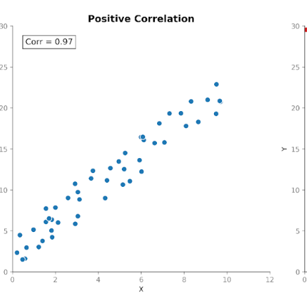
This standardized scale makes correlation easier to interpret than covariance. If we see a value of 0.8, we can immediately know that there is a strong relationship between the variables, regardless of what units were used in the original measurement.

This standardization also allows meaningful comparisons across datasets, features, and domains. This is why correlation is so commonly used in exploratory data analyses and feature investigations.

Covariance vs. Correlation: Key Differences

Covariance and correlation describe related properties of variable relationships, but they serve different analytical purposes.

In practical terms, covariance reflects raw co-variability, while correlation reflects that same relationship in standardized form. Understanding this distinction helps determine which measure better suits a given analytical task.

Covariance vs. Correlation Example

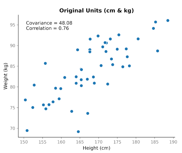
Suppose we collect data on two variables: height and weight. We expect them to be related, since in general taller people tend to weigh more. When we plot height in centimeters against weight in kilograms, we see a clear upward trend. As height increases, weight tends to increase too.

When we calculate the covariance, we get a positive value: 48.08. The fact that it’s positive tells us the two variables move in the same direction. When height is above average, weight is usually above average as well.

Now here’s where it gets interesting. Let’s take the exact same data and change the units. We’ll convert height from centimeters to meters, and weight from kilograms to pounds. The people haven’t changed. The relationship hasn’t changed. The pattern in the scatterplot looks the same. But when we recalculate the covariance, the number is different: 1.06. It’s still positive, but the magnitude is very different. And the only thing we changed was the units.

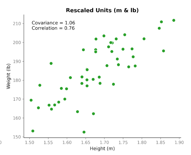
This shows an important property of covariance: it captures direction, but its magnitude depends on scale. If we stretch or shrink one of the variables by changing units, the covariance stretches or shrinks too.

Now, let’s look at correlation using the same data before and after the unit conversion. The correlation using centimeters and kilograms is 0.76. After converting to meters and pounds, it’s still 0.76.

Unlike covariance, correlation adjusts for the variability in each variable before measuring the relationship between them. Because of that adjustment, the value does not change when we switch units. It focuses only on how tightly the points follow a linear pattern and whether that pattern slopes upward or downward.

This simple example highlights the main difference between these metrics: covariance reflects both direction and scale, whereas correlation reflects relationship strength independent of scale. In practice, this means correlation is more reliable for comparing relationships across variables measured on different scales, while covariance is more relevant in contexts where the magnitude of variability matters, such as modeling.

Covariance Can Be Hard to Interpret

As we’ve discussed, covariance tells us whether two variables move in the same direction, but its magnitude is difficult to interpret.

The main issue is that covariance depends on the scale of the variables, not just their relationship. If the values of one or both variables are larger or more spread out, the covariance will also tend to be larger.

This sensitivity comes from two sources. The first is the units of the data. Changing units changes the covariance. Measuring income in dollars versus thousands of dollars produces very different covariance values, even though the relationship is identical.

The second source is the amount of variability in the variable. Even when units stay the same, a dataset with a wider range or greater spread will typically produce a larger covariance than a tighter dataset with the same underlying relationship. A large covariance does not necessarily indicate a strong relationship. It may simply reflect larger scales or greater variability in the data.

Because of this sensitivity to scale, covariance is often used internally, like for fitting models, instead of being reported directly.

Why Correlation Is Used More Often

Correlation addresses many of the interpretability challenges of covariance by standardizing the relationship between variables. Because correlation values are always between −1 and +1, the magnitude is immediately meaningful: values close to 1 or −1 indicate strong linear relationships, while values near 0 indicate weak or no linear relationship. This standardization also allows for direct comparison across variables or datasets, making correlation easier to communicate and interpret.

These properties make correlation particularly useful for exploratory data analysis, inspecting relationships between features, detecting redundancy or multicollinearity, and reporting findings. Correlation matrices and heatmaps are also useful as first-pass tools when examining datasets.

That said, correlation is not a complete replacement for covariance. Because correlation removes the effects of scale, it reflects only the strength of the relationship, not the raw variability. In modeling contexts, such as principal component analysis or multivariate statistical models, the original scale captured by covariance can be important for understanding variance structure and guiding algorithm behavior.

A Linear Algebra Perspective

So far, we’ve looked at covariance between variables one pair at a time. Linear algebra shows us how to scale that idea up to the whole dataset at once. We can do this by arranging our data into a matrix.

In a basic data matrix, each row represents an observation, and each column represents a variable. To understand relationships between variables, we can first center the data by subtracting the column’s mean from each value. This step ensures that we are focusing on deviations from typical values rather than absolute values.

Multiplying the centered data matrix by its transpose produces a structure that captures how variables move together. This product, after scaling, is the covariance matrix. From a linear algebra perspective, the covariance matrix summarizes how variability is distributed across the dimensions of the dataset.

Thinking about covariance in this way helps explain why it appears so frequently in data science. Many algorithms, including principal component analysis (PCA) and other dimensionality reduction techniques, rely on this matrix representation to understand patterns and structure in the data. Conceptually, the covariance matrix provides a map of how different dimensions of the dataset interact.

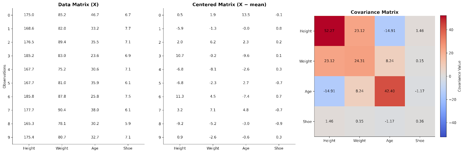
Here we can see data for four variables arranged in a data matrix. It is then centered and used to make a covariance matrix.

If you’d like a deeper dive into linear algebra for data science, check out our Linear Algebra for Data Science in R course, which covers the foundations you need to understand matrix-based approaches like covariance.

Covariance and correlation matrices

The covariance matrix summarizes how variables move together across an entire dataset. In practice, we often examine these relationships using either covariance or correlation matrices, depending on whether we want to preserve the original scale or standardize the results.

A covariance matrix contains the covariances between all pairs of variables. The diagonal numbers show the variance within each variable, while the off-diagonal numbers reflect how variables change together. Because covariance preserves the original scale and units of the data, the matrix captures the raw structure of variability. This makes covariance matrices particularly useful in modeling workflows and multivariate analyses.

A correlation matrix, on the other hand, standardizes these relationships. Each diagonal entry equals 1, since every variable correlates exactly with itself. All off-diagonal values lie between −1 and +1, showing the correlation between variables. By removing scale effects, correlation matrices are easier to interpret by humans and allow direct comparison across variables. They are especially useful in exploratory data analysis and for quickly identifying strong or weak linear relationships among features.

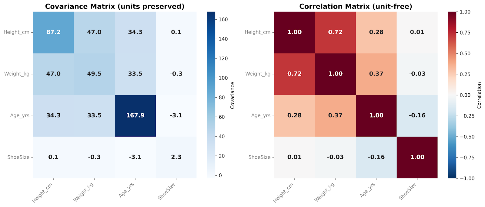
In these matrices, we’re comparing four variables with each other. I like to add a heatmap overlay when presenting these matrices. The color of each cell helps us see, at a glance, the relative magnitude of the covariance or correlation values.

How to Convert Covariance to Correlation

Conceptually, correlation is derived from covariance by standardizing the relationship between variables. You simply divide the covariance by the standard deviation of each variable. This scaling removes the units and the magnitude of the variables, producing a standardized measure that always falls between −1 and +1. This transformation is why correlation values are directly comparable across different variables or datasets.

In practice, converting covariance to correlation is done automatically in most statistical software, so analysts rarely need to calculate it manually. However, it’s always important to understand what your software is doing behind the scenes. For example, understanding how covariance is converted into correlation explains why you can’t convert in the opposite direction(at least not without information for the standard deviation of both). Correlation no longer contains the units or the magnitude information necessary to convert to covariance.

When to Use Covariance and Correlation

Covariance is most useful when the scale and units of the data are meaningful or when you need the raw structure of your data’s variability. It is commonly used in multivariate modeling, probabilistic models, and in constructing covariance matrices for linear algebra–based methods. In these contexts, preserving the original variability allows algorithms to capture the true structure of the data and understand how dimensions vary together.

Correlation, by contrast, is better suited for human interpretation, comparisons between datasets, and exploratory analyses. I like to use this metric in visualizations, such as heatmaps so I can see and communicate these relationships at a glance. Because correlation standardizes the relationship, it’s also helpful in preparing your data for techniques where treating all features on a comparable scale can be important.

Covariance vs. correlation in data science and statistics

Often, both measures appear in the same workflow. Covariance matrices form the mathematical foundation of many multivariate techniques because they retain the original variability of the data. Correlation matrices, on the other hand, are frequently used during exploratory stages to understand the dataset’s structure before modeling.

Some models can use either statistic, depending on the goal. Consider principal component analysis (PCA). When PCA is performed on a covariance matrix, variables with larger variance naturally exert more influence on the resulting components. This can sometimes be desirable if differences in scale reflect meaningful differences in variability. For example, if you are analyzing daily stock returns, a more volatile stock may appropriately shape the principal components because that variability reflects real market behavior.

Using a correlation matrix instead standardizes the variables before decomposition. Each feature is placed on the same scale, so no variable dominates simply because it has larger units or a wider numeric range. This approach may be more appropriate when variables are measured in different units, such as height (cm), weight (kg), blood pressure (mmHg), and cholesterol (mg/dL).

Neither approach is universally better. The appropriate choice depends on whether scale differences reflect meaningful structure or are simply artifacts of measurement.

Common Misconceptions About Covariance and Correlation

One common misconception is that a high covariance automatically indicates a strong relationship. However, large covariance values may simply reflect the scale or variability of the variables rather than the strength of their relationship. If you want to know the strength of the relationship, you really need to standardize it by looking at the correlation.

You have probably heard the phrase “correlation does not imply causation” close to a million times! And yet, it is still probably the most common misconception I run across. It is understandable to look at a strong correlation and assume there is a causal link. It’s a shortcut our brains have used for millennia to keep our ancestors alive. However, as data practitioners, we must resist this brain shortcut and recognize that correlation alone is not enough to prove a causative effect. Correlation measures association, not causal influence, and external factors may drive both variables simultaneously.

Another very common misconception is that covariance and correlation are basically the same thing. However, they are not interchangeable. While correlation is derived from covariance, it standardizes the relationship, making it a decidedly different metric that is not always a suitable substitute for covariance in calculations.

Lastly, it’s important to remember that these statistics only evaluate linear relationships. Nonlinear patterns may exist even when correlation and covariance is low or near zero, so relying on these statistics alone can overlook important structure in the data. I always recommend you plot your data and look at it before trying to interpret statistical measures. This can really save you if there is an obvious nonlinear relationship.

Pro Tips for Interpreting Relationships Between Variables

First, always consider your measurement’s scale. Differences in units or variability can affect raw measures like covariance, so it’s important to know what your numbers represent.

Second, figure out what you need from your data. Covariance is most useful when preserving the raw variability is important. This is often the case in modeling or when constructing covariance matrices for multivariate analyses. In these contexts, the magnitude of variation carries meaningful information. But if you don’t need that raw variability, you might prefer the standardization and interpretability of correlation.

Thirdly, always, always, always plot your data and look at it! Visual inspection can help guide your analyses and complements statistical summaries. You can use scatter plots to help you spot pairwise patterns, or matrices to get a quick overview of many variables at once.

Lastly, think about the downstream implications of your measurement choices. Choosing between a raw measure like covariance and a standardized measure like correlation will influence your modeling outcomes and interpretations. So make sure you align your selection with your analytical goals.

Conclusion

Covariance and correlation are closely related measures that describe how variables move together, yet they serve distinct purposes: covariance preserves original scale, while correlation standardizes for comparison.

If you’re interested in learning more about exploring your data, check out the Python Exploratory Data Analysis Tutorial. To learn how to figure out if your correlation really does show causation, check out Hypothesis Testing in R.