Least Squares Method: How to Find the Best Fit Line

Imagine you're trying to predict housing prices based on square footage. You have data points from recent sales, but they don’t form a perfect pattern. Some homes sell for more than expected, and others sell for less. How do you find the best trend line that reflects the overall relationship between size and price without letting individual homes throw off your prediction?

The least squares method might be just the solution you need. In this article, we will explore the core concepts of the least squares method, its variations, and applications. By the end, you will have a solid understanding of how to use this method and apply it to real problems.

What Is the Least Squares Method?

The least squares method is a statistical technique used to determine the best-fitting line or curve for a set of data points. It works by minimizing the squared differences between the observed and the predicted values in a dataset. The difference between the actual data points and the values predicted by the model are called residuals. The goal is to find a model that minimizes the sum of these squared residuals, leading to the most accurate predictions possible.

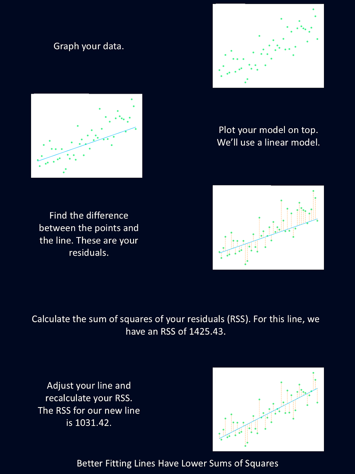
The diagram above gives a brief explanation of the steps of the least squares method.

This method was derived by 18-year-old Carl Friedrich Gauss in 1795 (you may recognize his name from the Gaussian distribution). Adrien-Marie Legendre later formalized the technique in 1805 and was the first to write a paper using the least squares method in order to reconstruct the orbit of an asteroid. 

How the Least Squares Method Works

The least squares method finds the line that fits a set of points the best by minimizing the sum of the squared differences between the observed values and the predicted values. This is used to find the model parameters with the closest fit possible.

Let’s try this with an extremely small dataset: only 10 points. First, we need to choose a model to fit our data. For this simple example, we’ll choose a simple linear regression, which means we are performing a regression where we only have exactly one independent and one dependent variable.

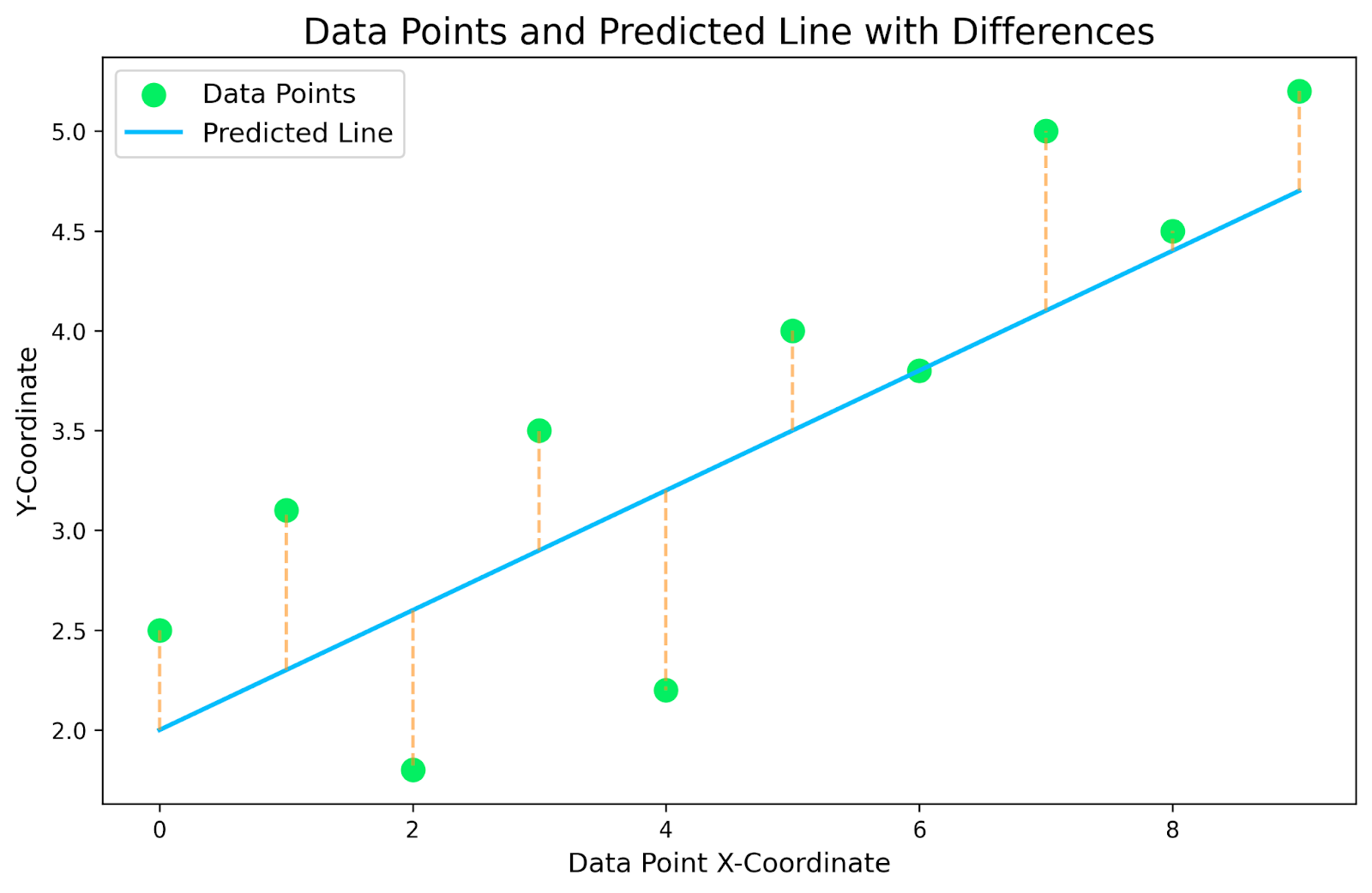
The above graph is a plot of our small dataset, with a linear regression plotted on top. The yellow dotted lines connecting the data points with the predicted line are the residuals. The goal is to find the linear regression model that minimizes these yellow dotted residual lines.

For each data point in our dataset, we need to find the difference in y-coordinates between the data point and the line. These will be our residuals. We then square each residual to remove any negative numbers and take the total sum. This will give us a sense of how well our line fits our data. Check out the table below for the breakdown for our specific graph.

Now that we have an idea of how well this line fits our data, we can tweak the parameters of the line, either its slope or its intercept, and rerun our calculations. The line that has the lowest sum of squared residuals is the line that best fits our data. Therefore, that line will give us the best predictions.

Using least squares method to find the best line

In the above example, we didn’t find the best fitting line. Instead we just calculated how well that line fit the data. Now we could iterate through a bunch of potential lines and perform the same calculation to find the ones that fits the best. Or we could use a little bit of algebra to find the best line more quickly. Let’s try that.

We’ll start with the equation for the linear regression: y=mx+b, where b is the y-intercept and m is the slope. Now let's make up some data.

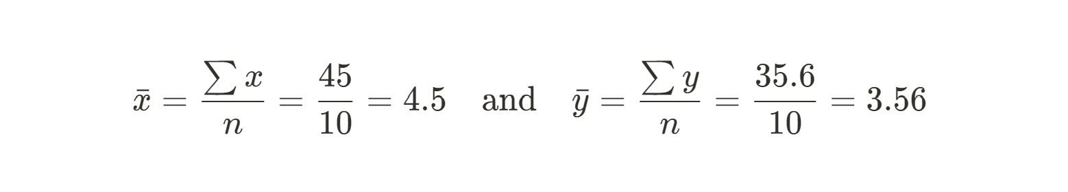
First, we need to calculate the mean of the X and Y values. These will serve as our predicted values:

Next, we can use the sum of the squares of our residuals between each data point and our predicted value (the mean) to find the slope. Here’s the equation we’ll use:

Since this is a pretty wieldy equation to do by hand, we’ll calculate the numerator and denominator separately. Let’s start with the numerator:

Now let’s do the same for the denominator:

Now we can calculate the slope for our best fit line.

So now we know the slope for the line that will fit our data the best. Next, we need to find our y-intercept. The formula for the intercept b is easy to find using a little bit of algebraic rearranging:

Since we already know the slope, we can simply insert our mean x and y and solve for b.

Now that we have both m and b, we can write the equation of the best-fitting line:

The least squares method allowed us to quickly and easily derive the best linear regression line, even by hand! Obviously the more data you have, the harder this will be to do by hand. Fortunately, since the math is fairly straightforward, it’s very simple to implement this method in Python or R. For detailed explanations on how to do this, check out Essentials of Linear Regression in Python and How to Do Linear Regression in R.

Mathematical foundations of the least squares method

Above, we used an example with simple linear regression and found the slope and intercept using nice closed-form equations, and we modeled the dependent variable as a function of the independent variable: y=mx+b.

However, the equations I showed above only work when you have one independent variable. Another way to find the coefficients for a regression is to use what is known as the normal equation, which provides a matrix-based solution to the least squares problem. The normal equation refers to the matrix equation that results from minimizing the sum of squared residuals using the least squares method. Geometrically, and using the language of linear algebra, the least squares solution can be visualized as the orthogonal projection of the observed data vector onto the column space of the model matrix. Put simply, this just means that the errors are minimized in a way that ensures the predicted values lie as close as possible to the observed data, given the constraints of the model.

In cases where the matrix is not invertible (which means the system of equations does not have a unique solution), the Moore-Penrose pseudoinverse provides a way to compute a least squares solution. This gives us the flexibility to handle situations where the system is underdetermined (which means there are more unknowns than equations) or overdetermined (which means there are more equations than unknowns).

If you need a refresher on matrix algebra, I recommend the Linear Algebra for Data Science in R course.

Types of Least Squares Methods

So far, we’ve only talked about using the least squares method with an ordinary least squares estimator. However, it is a versatile tool that can be adapted to many scenarios depending on the nature of the problem you’re tackling. Let’s explore a few types of least squares methods, what makes them unique, and their practical uses.

Linear least squares

By this point, you should be pretty familiar with linear least squares (also referred to as ordinary least squares). It is used with models that have linear coefficients, such as in simple or multiple linear regression. The goal is to find the line (or hyperplane, in the case of multiple linear regressions) that minimizes the sum of squared residuals.

This type of least squares assumes the residuals have a constant variance and there are no significant outliers in the data. It can be applied to most things that have a linear relationship. For example, you might use this for relationships between gestation length and birth weight or between ad spending and sales revenue. This is the type of least squares I most often use and that I most often hear others talk about.

Weighted least squares

Weighted least squares is an extension of this method that works when the variance of the residuals is not constant. By assigning weights to each data point, weighted least squares gives more importance to observations with lower variance. The equation for this is similar to the previous sum of squares, but with a weight (w_i) applied to each residual:

This method is useful for datasets where the measurement error varies between observations, for example in calibrating sensors. Weights are typically the inverse of the variance for each observation.

Robust least squares

Robust least squares is designed to handle datasets with outliers that can disproportionately influence the results of ordinary least squares. It uses iterative reweighting techniques to reduce the impact of outliers.

In robust least squares, you can use methods like least absolute residuals (LAR) or bisquare weights to iteratively adjust weights and downplay the influence of outliers.

An example of when you might use this is with financial modeling, where you want to account for extreme market crashes. If you have a dataset where you don’t want to remove the outliers, but you still want to account for them, robust least squares may be the path to take.

Nonlinear least squares

Least squares is not only for use with linear regressions. A nonlinear least squares is used when the model you’re applying is nonlinear in its coefficients. This is more complicated than linear least squares, and can require iterative optimization techniques (like Gauss–Newton or Levenberg–Marquardt) to find the best fit.

It’s important to be careful with nonlinear least squares. The calculation can be sensitive to initial parameter estimates as well as to convergence issues. Examples of when you might use this include modeling the exponential growth of viruses in a body during infection or modeling chemical reaction rates in the lab.

Total least squares

Up until now, we’ve mostly been talking about instances where only the dependent variable has errors. And we’ve been minimizing the vertical distances between the our model and our data. But what if you have errors in your independent measurements too?

Total least squares is useful when both the independent and dependent variables have measurement errors. This method accounts for errors in all variables. This can be especially useful in fields like astronomy and geodesy (the field which measures Earth’s shape and gravity field), where measurement errors are present in all dimensions due to the high level of precision necessary. Total least squares is often used in conjunction with singular value decomposition.

Generalized least squares

Generalized least squares is an extension of the least squares method that addresses the challenges posed by correlated residuals. With generalized least squares, we transform the data into a form where ordinary least squares can be applied. This transformation involves using the covariance matrix of the residuals to account for their correlation structure, allowing for more accurate parameter estimates.

This can be particularly useful in situations like time series analyses, where residuals may exhibit autocorrelation. 

Applications of the Least Squares Method

The least squares method is a widely used statistical technique with applications across numerous fields.

In statistics and data science, least squares is used to build linear and nonlinear regression models to make predictions based on known inputs. It is also useful in analyzing trends, particularly in time series data.

In finance, least squares is used in stock performance analysis, helping to determine the relationship between a stock's performance and market indices. For example, it can be used to calculate a stock’s sensitivity to market movements. It also helps with risk modeling by fitting models to historical financial data to estimate risk and return.

Engineers use least squares in sensor calibration to fit models to observed data and minimize measurement errors. It is also applied in signal processing for filtering and noise reduction, allowing for clearer data interpretation.

Of course, least squares got its start in astronomy; its first use was by Carl Friedrich Gauss to predict the orbit of the asteroid Ceres. It’s also used in geodesy in modeling the Earth's shape based on observational data, which is essential for accurate geographical measurements.

If you’ve dabbled in machine learning, you’ll recognize the least squares method as a method for minimizing the loss function during the training of linear regression models. You may have also used it during feature selection to identify the most important variables contributing to the model.

It has a role in many of the other hard sciences as well, such as physics and chemistry. It can be used to fit curves to experimental data, such as reaction rates or physical measurements, and help minimize errors in experimental setups.

The least squares method is a versatile statistical tool. Personally, I’ve used this method to calibrate pressure sensors, make predictions based on my experimental data, and during machine learning training. The ability to reliably model relationships and minimize errors is a feature that offers value to many different disciplines.

Assumptions and Diagnostics

The least square method makes some key assumptions about your data and the model being used. It’s important to understand these assumptions, because violating them can lead to biased or unreliable results. So, let’s discuss these assumptions, as well as how to diagnose and address potential issues.

One assumption is the independence of errors, which means that the residuals should not be correlated. If errors are correlated with each other, particularly in sequential or spatial data, estimates can become distorted. The Durbin-Watson test can detect autocorrelation in residuals, especially for time-dependent datasets. If you do find a correlation, you can use the generalized least squares to account for it.

Another assumption is that the variance of the residuals remains constant across all levels of the independent variable. If residuals display a funnel-shaped spread when plotted against fitted values, this assumption is likely violated. To address this issue, you can use the weighted least squares to assign appropriate weights to your observations. Alternatively, you can use transformations like logarithmic or square root adjustments to stabilize unequal variance and fix any issues of heteroscesdasticity.

As with all modeling, it’s important that the structure reflects the underlying relationship between the variables. If it doesn’t, it doesn’t matter how optimized your fit is; the results will still be misleading. Residual plots and goodness-of-fit metrics like R^² can help you determine whether your chosen model captures the patterns in the data. 

The standard least squares method assumes that independent variables are measured without error. So it’s important to know the precision of your independent measurement. You should have an idea of the precision of this measurement by looking at the collection methods. If measurement errors do exist in your predictor, be sure to use the total least squares method to mitigate inaccuracies in your modeling.

Finally, the distribution of residual errors plays a significant role, particularly in hypothesis testing and confidence interval estimation. Least squares assumes that errors follow a normal (Gaussian) distribution, and deviations from normality can affect inference. Histograms and Q-Q plots help assess whether residuals align with expected distributions. If you have significant departures from normality, robust regression techniques or bootstrapping methods can provide more reliable estimates that are less sensitive to outliers.

Advantages and Disadvantages of Least Squares

The least squares method is a widely used tool in data analysis. But that doesn’t mean it should be used for every dataset.

The least squares method offers several advantages. It’s fairly easy to compute, especially for linear models. It is easily interpretable by both technical and non-technical audiences. Plus, there are different styles, such as weighted, robust, and nonlinear regression, which makes it highly versatile. And importantly, it has a strong theoretical foundation provided by the Gauss-Markov theorem. All this makes least squares broadly applicable and used in fields ranging from economics to engineering.

However, the method is sensitive to outliers, which can disproportionately affect the model's results. It also assumes there are no errors in the predictors, which may not hold true in real-world data. Additionally, least squares can be limited by multicollinearity. Which means highly correlated predictors can lead to unstable coefficients and therefore unreliable estimates. It also requires constant variance of residuals, a condition that may not always be met.

It’s important to closely examine your dataset and your goal before you decide that the least squares method is the best tool for your circumstance.

Conclusion

The least squares method is a fundamental tool for any data analyst. By finding the best fit for our data, we can make more accurate predictions and find more insightful trends.

For further reading about measuring straight lines in Euclidean space, I recommend our Understanding Euclidean Distance: From Theory to Practice tutorial. Also, make sure to enroll in our regression courses to really become an expert. 

• Introduction to Regression with statsmodels in Python
• Introduction to Regression in R