Time Series Decomposition: Understand Trends, Seasonality, and Noise

Decomposition is one of the more interesting things in data science. At its core, decomposition is about breaking something that is complex into more simple, more interpretable parts. This can happen to a matrix, a model, or a signal. 

Because it’s a general idea, it can take a lot of forms. In linear algebra, there are QR decomposition, eigendecomposition, singular value decomposition, and Cholesky decomposition, to name a few. In other domains, there’s the Fourier transform, principal component analysis,  and even topic modeling using methods like LDA. The variability in regression models can be decomposed into sum of squares components: SST, SSR, and SSE. We can even think of decision trees as a form of decomposition. 

Here, we will review one of our favorites: time series decomposition. If, at the end, we’ve piqued your curiosity about it, take our Forecasting in R course with Professor Rob Hyndman.

What Is Time Series Decomposition?

Time series decomposition is a method used to break down a time series into separate components called trend or trend-cycle, seasonality, and residuals. The purpose of time series decomposition is to better understand the underlying patterns and improve forecasting accuracy.

What Are the Components of a Time Series?

Let’s take a look at the time series components. This might be the best way to understand the idea.

Trend component

The trend of a time series (as the name suggests) is the long-term movement. We should say that the trend component is often actually thought of as the trend-cycle, where cycles are understood to be long, irregular patterns. Car sales were historically understood to move in seven-year cycles (for whatever reason) although probably, with the movement towards electric cars, not anymore.

The big takeaway that people get from the trend is usually this: Is the data increasing or decreasing, or remaining stable, over the long run? A global rise in ocean temperatures over the last few decades is one clear (read: bad) trend.

Seasonal component

The seasonal component is going to take a little bit longer to explain because it’s a bit more complicated. The seasonal component of a time series is the repeating short-term cycles in the data that occur at regular intervals. Think daily, monthly, weekly, quarterly. The key here is that the intervals have to be pretty regular. You might see, for example, that coffee shop orders follow a weekly seasonality if people like to make coffee at home on Sundays. (We will explore this question about coffee shop orders in the next section.)

The thing about seasonality is that it can be more complicated than it seems. Think about how the number of weeks in a year is not an integer (~52.18). Or think about how the months are not spaced evenly: February has 28 (or 29) days, but July always has 31.

What is more, since every year has a little bit more than 52 weeks, and since months also vary, you can’t divide most months evenly into weeks. This is obvious when you study a calendar. But what is less obvious for a data analyst is that, when you’re looking at data at the weekly level, then aggregating it to the monthly level, you may see inconsistent things, like how one January might have four Mondays, but the next might have five.

The residual / irregular / remainder component

Everything that is left over after pulling out the trend-cycle and the seasonal component we call, appropriately, the residual component, which includes anomalous things in the data, like a big event, and random noise. Contrary to what you might think because of how it sounds, the residual component is not a useless artifact. All data have unexplained variability, and quantifying the size of that variability is important. Interestingly, residuals often take the shape of a Gaussian distribution in a well-behaved series, in which case we might evaluate black swan events with hypthothesis tests.

Time Series Decomposition Models

Now that we have covered the constituent parts of a time series, we should now mention that there are actually two different general types of time series decomposition. We will start with the additive model.

Additive decomposition

Here is the formula for additive decomposition:

Note the plus signs. What this formula is saying is that if you take the trend and add it to the seasonal component, and add that to the residuals, you get back the original time series. Generally speaking, we use an additive decomposition when seasonal variation is constant over time.

Multiplicative decomposition

Here is the formula for multiplicative decomposition. Note the multiplication signs in this version. 

We use a multiplicative model when seasonal variation scales with the trend. That is, when you see that the size of the seasonal effects become larger as the overall series moves up or down. What we're describing here is really a form of heteroscedasticity.

Time Series Decomposition Techniques

So far, we have covered what goes into a time series decomposition, and the two main general types. Moving forward, we need to talk about the two most common methods. Each of these can be applied as an additive or multiplicative model. 

Classical decomposition

Classical decomposition is the easier one to understand. It’s from the 1920s but still relevant today. To show classical decomposition, let’s use Excel. Classical decompostion, like STL, which we will show next, can be done with either an additive or multiplicative model. For this example, we will create an additive version.

If you want to try for yourself, use the index_1 CSV in this very interesting coffee sales dataset you can find on Kaggle. For your reference, we aggregated and summarized the sales by day.

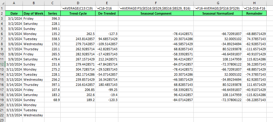
• First, we calculate the trend-cycle. We are identifying a weekly seasonality, and there are seven days in a week, so the seasonal period is odd, which means our moving average should be centered using a symmetric window. That is, a 7-day moving average. Do be careful with alignment and centering in the Excel sheet.

• Next, we find the detrended series by subtracting the trend from the original.

• Then, to find the seasonal component, we average the detrended values for each seasonal period. An important addition: You will see that the seasonal component likely does not sum to exactly zero. Make sure to adjust for this with normalization:

  • Calculate the mean of your seasonal component.

  • Subtract the seasonal mean from every seasonal value.

• Finally, for the remainder, we subtract the trend and seasonal period from the original series. 

If we saw that our series had a seasonal effect that changed with the data level, we would have considered a multiplicative decomposition instead. The steps for multiplicative decomposition are much the same, except that we use division instead of subtraction. Specifically, we would find the detrended series by dividing the original series by the trend-cycle. Then, later, to find the remainder, we would divide the original series by the product of the trend and seasonal components. (Alternatively, we could have taken the natural logarithm of the original series and applied an additive decomposition. This would be functionally the same.)

STL decomposition 

STL decomposition, which stands for seasonal and trend decomposition using LOESS is a more modern version of decomposition. It's harder to explain, but it's generally more flexible than the classical method. STL works by using a method called LOESS, which fits simple regression models to small overlapping chunks of the data. It applies this locally weighted regression to isolate the trend and seasonal components separately.

This method addresses specific drawbacks in classical decomposition, namely that, in the classical version, no trend-cycle or remainder estimates are available for the first and last observations. You can see this in the blank Excel spaces, in rows 3, 4, 5, and 20, 21, and 22, above.

We should also say the trend-cycle as identified by classical decomposition smooths out rapid rises and falls, so it might gloss over important things happening in the series. Finally, classical decomposition takes for granted the idea that there is a seasonal pattern but, given enough data, we can sometimes see the seasonal pattern change.

Let's start by creating a time plot of the original series. Like before, as a first step, we are aggregating and summarizing the Kaggle dataset to get the series we are interested in.

coffee_sales_data <- read.csv("/Users/x/Desktop/index_1.csv")
coffee_sales_data <- as.data.frame(coffee_sales_data)

library(dplyr)
library(ggplot2)

coffee_sales_data |>
  group_by(date) |>
  summarize(money = sum(money)) |>
  ggplot(aes(x = as.Date(date), y = money)) +
  geom_line(color = '#01ef63') +
  labs(title = "Coffee Sales") +
  labs(subtitle = "Time series")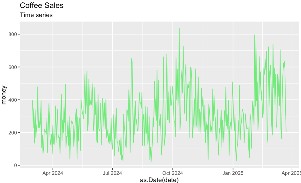

Next, we decompose our series into trend, seasonal, and remainder components. The box at the top of the decomposition graph shows the original series, if a little squished.

coffee_sales_data |>
  group_by(date) |>
  summarize(money = sum(money)) |>
  mutate(date = as.Date(date)) |>
  as_tsibble() |>
  filter(date > '2024-02-28') |>
  filter(date < '2024-05-01') |>
  model(
      STL(money ~ season(window = "periodic"))
  ) |>
  components() |>
  autoplot(color = '#203147') +
  labs(title = "Coffee Sales") +
  labs(subtitle = "Classical additive decomposition")

coffee_sales_data |>
  group_by(date) |>
  summarize(money = sum(money)) |>
  mutate(date = as.Date(date)) |>
  as_tsibble() |>
  filter(date > '2024-02-28') |>
  filter(date < '2024-05-01') |>
  model(
      STL(money ~ season(window = "periodic"))
  ) |>
  components() -> ts_components

ts_components |>
  autoplot(color = '#203147') +
  labs(title = "Coffee Sales") +
  labs(subtitle = "Classical additive decomposition")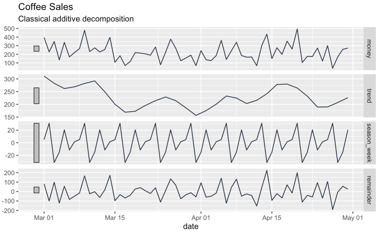

Notice that, unlike with classical decomposition, the dataframe that we get back has no gaps at the beginning or end.  

print(ts_components)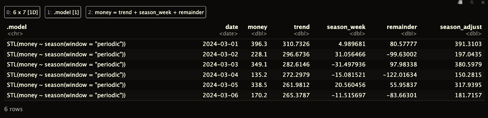

There are some drawbacks with STL decomposition, also, and, if you're interested, we have added that information into our FAQs. 

Time Series Decomposition and Seasonal Adjustments

Often, it’s helpful to create a seasonally-adjusted version of the data. Time series decomposition helps with this. To create a seasonal adjusted version, we simply add the trend and the remainder components together. Or else, we could subtract the seasonal component from the original series; both would arrive at the same thing.

seasonally_adjusted <- components |>
  mutate(seasonally_adjusted = money - season_week)

season_adjust_data <- seasonally_adjusted |>
  select(date, money, season_adjust) |>
  pivot_longer(cols = c(money, season_adjust), names_to = "series", values_to = "value")

season_adjust_data |>
  autoplot() + facet_wrap(~series) +
  scale_color_manual(values = c(
    "money" = '#203147',          # blue
    "season_adjust" = '#01ef63'   # orange
  )) +
  facet_wrap(~series) +
  labs(title = "Coffee Sales: Original vs Seasonally Adjusted")

We are discovering that there is not especially strong seasonality in this particular dataset, which itself is interesting.

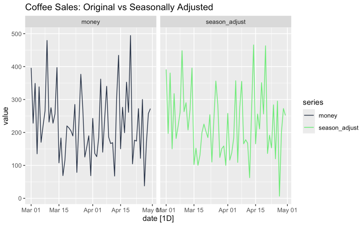
The power of seasonal-adjusted data is that it can help us understand certain features of our series. We can see if the underlying trend is the result of seasonality, for one. For two, we can more closely examine unusual occurrences in the data. Do we think our Friday promotion worked because it was a Friday or because it was a promotion? Well, using time series decomposition and seasonal adjustments, we can test questions like that.

Time Series Decomposition and Forecasting

You might be surprised to hear that time series decomposition is also helpful in forecasting. We think about this in two main ways. First, we want to understand our time series components to help us decide which forecasting model we should use. If we see strong seasonality, we might lean toward models like Holt-Winters exponential smoothing or ETS methods, which are specifically built to handle both trend and seasonal components.

Secondly, we can even use decomposed data as part of our forecasting, which gives us options. We can, for example, run a non-seasonal forecasting model on a seasonal-adjusted version of our data. (We can reintroduce the seasonal component later.) Seasonal adjustment is especially helpful when we want to use flexible models, like standard ARIMA and linear regression. 

Here, we create a simple ARIMA model to forecast the seasonal-adjusted data. 

season_adjust_data_filtered <- season_adjust_data |>
  filter(series == "season_adjust") |>
  as_tsibble(index = date)

seasonal_adjust_arima_model <- season_adjust_data_filtered |>
  model(
    ARIMA(value)
  )

seasonal_adjust_arima_model |>
  forecast(h = "14 days") |>  
  autoplot(season_adjust_data_filtered, color = '#01ef63') +
  labs(title = "Forecast of Seasonally Adjusted Coffee Sales",
       subtitle = "Simple ARIMA Model",
       y = "Money (Seasonally Adjusted)",
       x = "Date")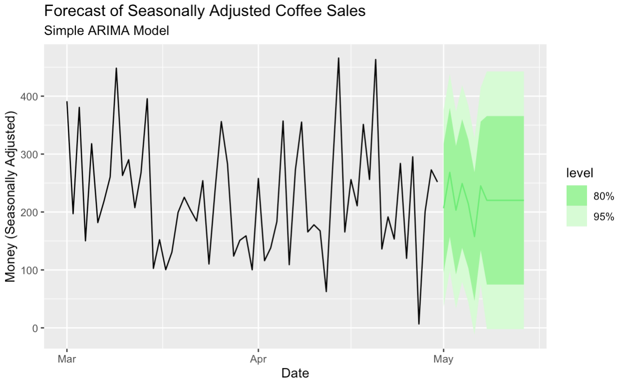

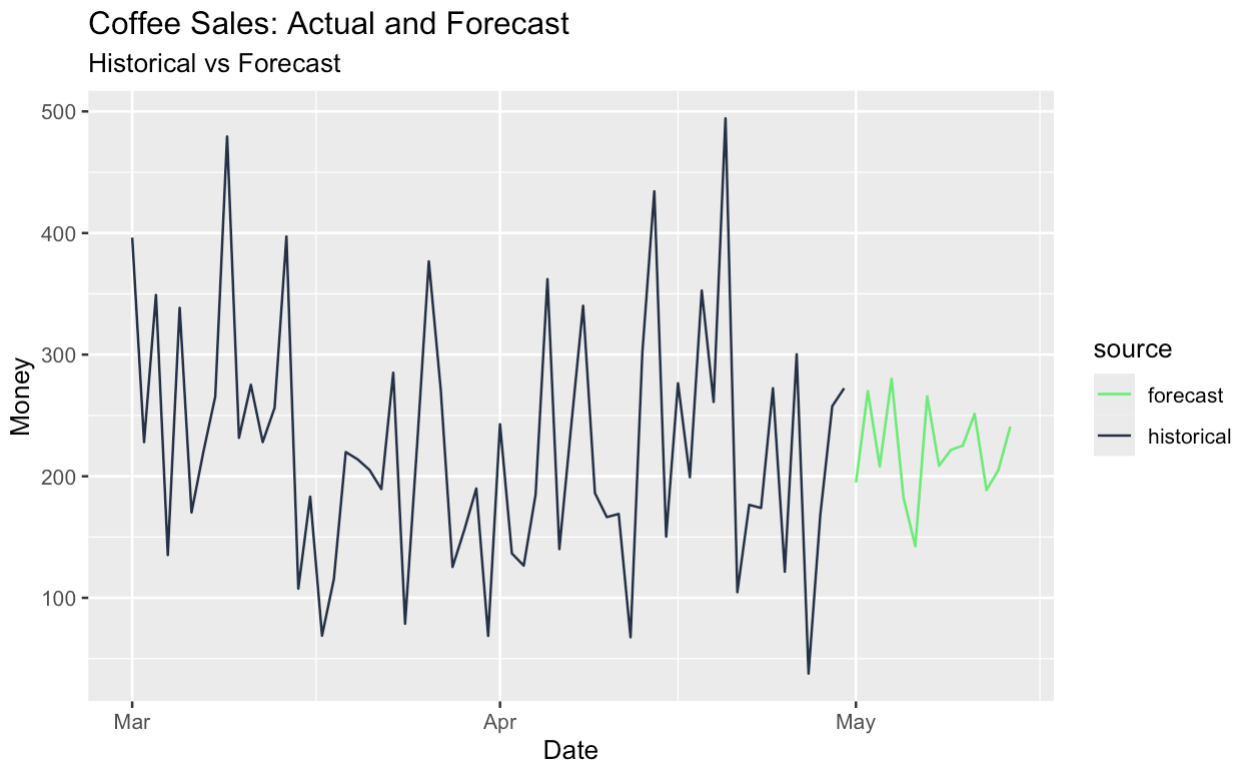
We can also forecast the seasonal-adjusted series and add the seasonal component back in, which effectively gives us a seasonal forecast. All this has been made possible through our original decomposition.

# Build tagged historical and forecast data
historical_data <- components |>
  as_tibble() |>
  select(date, money) |>
  mutate(source = "historical")

forecast_data <- final_forecast |>
  as_tibble() |>
  transmute(date, money = money_forecast) |>
  mutate(source = "forecast")

# Bind and create tsibble
full_data <- bind_rows(historical_data, forecast_data) |>
  as_tsibble(index = date, validate = FALSE)

# Plot with color by source
full_data |>
  ggplot(aes(x = date, y = money, color = source)) +
  geom_line() +
  scale_color_manual(values = c(
    "historical" = "#203147",   # dark blue for real data
    "forecast" = "#01ef63"      # green for forecast
  )) +
  labs(
    title = "Coffee Sales: Actual and Forecast",
    subtitle = "Historical vs Forecast",
    y = "Money",
    x = "Date"
  )

Final Thoughts

I hope you enjoyed our article on time series decomposition! Remember that decomposition is just one part of time series analysis, so to become an expert, enroll in our Forecasting in R course with Professor Rob Hyndman, who helped develop the R packages that we used for our visuals. We also have a Visualizing Time Series Data in Python course if you found the ideas in this article interesting but prefer Python, which is also very good for this kind of thing.