Mean Reversion: Something to Know for Statistics and Finance

Imagine you're watching the spread between two airline stocks, companies that tend to move together because they share the same fuel costs, routes, and passenger demand. One morning, the spread widens sharply: something idiosyncratic hit one ticker while the other barely moved. A quant trader looks at this and asks a very specific question: is that spread likely to narrow back, or has something structural shifted?

Mean reversion is the tendency of a variable to move back toward a long-run level after deviating from it. It underpins a wide range of time-series models and quantitative trading strategies, and it's the statistical engine behind an entire family of approaches known as statistical arbitrage. The critical thing to keep in mind, and this article will keep coming back to it: mean reversion is a property you test for, not an assumption you make about prices.

What Is Mean Reversion?

Mean reversion describes a dynamic tendency: when a variable drifts away from its equilibrium level, forces tend to pull it back. That equilibrium might be a long-run statistical mean, a fair value implied by fundamentals, or a cointegrating relationship between two series. A positive deviation (the value sitting above the mean) tends to be followed by a decline. A negative deviation tends to be followed by a rise.

What makes mean reversion interesting is what it implies about shocks. In a mean-reverting process, a shock is temporary. Its effect dissipates over time, and the series eventually returns toward equilibrium. That's very different from a random walk, where every shock is permanent, and the series has no "home" to return to. We'll get to that distinction properly in a moment.

How Mean Reversion Works

Here's the basic intuition. A variable fluctuates around an equilibrium level. A shock (an earnings miss, a policy surprise, a liquidity crunch) pushes it away from that level. The farther it moves, the stronger the restoring force may be. Over time, the shock's effect fades, and the variable drifts back.

Contrast that with a random walk. Each period's value equals last period's value plus a random shock, and that shock never goes away. There's no equilibrium to return to; the series just wanders. The difference matters enormously for forecasting: mean-reverting series are, at least in principle, somewhat predictable over longer horizons. Random walks are not.

How to Identify Mean Reversion

Moving from intuition to evidence requires statistical analysis. No single test is enough. You want multiple forms of evidence pointing in the same direction.

Plot the time series

Start visually. A mean-reverting series tends to oscillate around a relatively stable level rather than drifting persistently upward or downward. But visual inspection is easy to fool: a trending series can look mean-reverting over short windows, and a slow mean-reverting process can look almost indistinguishable from a random walk. The plot is a first pass, not a verdict.

Examine autocorrelation

Autocorrelation measures the correlation between a series and its own lagged values. In a mean-reverting process, the autocorrelation function (ACF) decays rapidly toward zero, reflecting the transient nature of deviations. By contrast, a unit-root process shows autocorrelation that persists near 1.0 even at long lags. The ACF plot can reveal this pattern — a quick drop-off is consistent with mean reversion, while a slow, linear decline suggests non-stationarity. That said, autocorrelation alone doesn't confirm stationarity. It's one piece of evidence.

Test for stationarity

The Augmented Dickey-Fuller (ADF) test is the standard starting point. It tests the null hypothesis that the series has a unit root, meaning it's a random walk. Rejecting the null suggests the series may be stationary, which is closely associated with mean-reverting behavior. A p-value below 0.05 gives you grounds to proceed, though not certainty.

Estimate the speed of mean reversion

If the tests support mean reversion, the next question is how fast it happens. The speed parameter (often denoted κ in continuous-time models, or θ in some parameterizations) tells you how quickly deviations decay. High speed means deviations shrink quickly; low speed means the process wanders quite a bit before returning. This matters practically: a very slow mean-reverting process may not be tradeable over realistic horizons.

Mean Reversion vs. Random Walk

This distinction deserves its own section because it's the one people get wrong most often.

A random walk has no long-run mean to revert to. Shocks are permanent. The series is non-stationary, meaning its statistical properties (mean, variance) change over time. Forecasting beyond the very short run is futile. A mean-reverting process is stationary (or at least trend-stationary): its properties are stable, shocks are transient, and longer-horizon forecasts carry real information.

Here's the trap: a price series that has returned to a particular level several times in history isn't necessarily mean-reverting. Wander long enough, and any random walk will revisit its starting value. The question is whether there's a structural pull back to equilibrium, and that requires testing, not pattern recognition.

Mean Reversion and Stationarity

Mean reversion and stationarity is another point of confusion. They're closely related, but they're not the same thing. Stationarity is a formal statistical property: a stationary process has a constant mean, constant variance, and autocovariance that depends only on the lag, not the time period. Mean reversion is a dynamic tendency, the pull back toward equilibrium.

Most mean-reverting models assume stationarity, and most stationary processes exhibit some form of mean-reverting behavior. But the relationship isn't perfectly one-to-one. A process can be stationary without especially strong mean-reverting dynamics, and the label "mean-reverting" sometimes gets applied loosely to processes that are only weakly stationary. Worth keeping the distinction clear when you're reading the literature.

Mean Reversion vs. Momentum

Mean reversion and momentum pull in opposite directions. Mean reversion assumes that unusually large moves are more likely to reverse. A stock that has fallen sharply relative to its historical range is expected (under this view) to recover, not because prices "must" revert, but because the deviation from fair value creates a return opportunity.

Momentum assumes the opposite: recent directional movement is more likely to continue. A stock that has risen strongly over the past twelve months is expected to keep outperforming.

The evidence for momentum is quite strong at medium-term horizons (one to twelve months), while mean reversion tends to show up more clearly at short horizons (days to weeks) and very long ones (multi-year). Markets can, and do, exhibit both behaviors simultaneously at different time scales. Neither is a universal law.

The Ornstein-Uhlenbeck Process

The standard continuous-time model for mean-reverting behavior is the Ornstein-Uhlenbeck (OU) process:

Each term does something specific. The κ(μ − X_t) part is the restoring force: when X_t sits above the long-run mean μ, the process gets pulled downward; when below, upward. The parameter κ controls how strong that pull is, the speed of mean reversion. The σ dW_t term adds random noise with volatility σ.

Simulating OU paths with different κ values makes the intuition vivid. With high κ, paths hug the mean tightly, and deviations collapse quickly. With low κ, paths wander broadly and look, over short windows, almost indistinguishable from a random walk. This is why estimating κ carefully matters: a statistically significant but tiny κ may not be actionable in practice.

Half-Life of Mean Reversion

The OU model gives us κ, but κ on its own is hard to reason about intuitively. The half-life translates that abstract speed into something concrete: the expected time for a deviation from equilibrium to shrink by half.

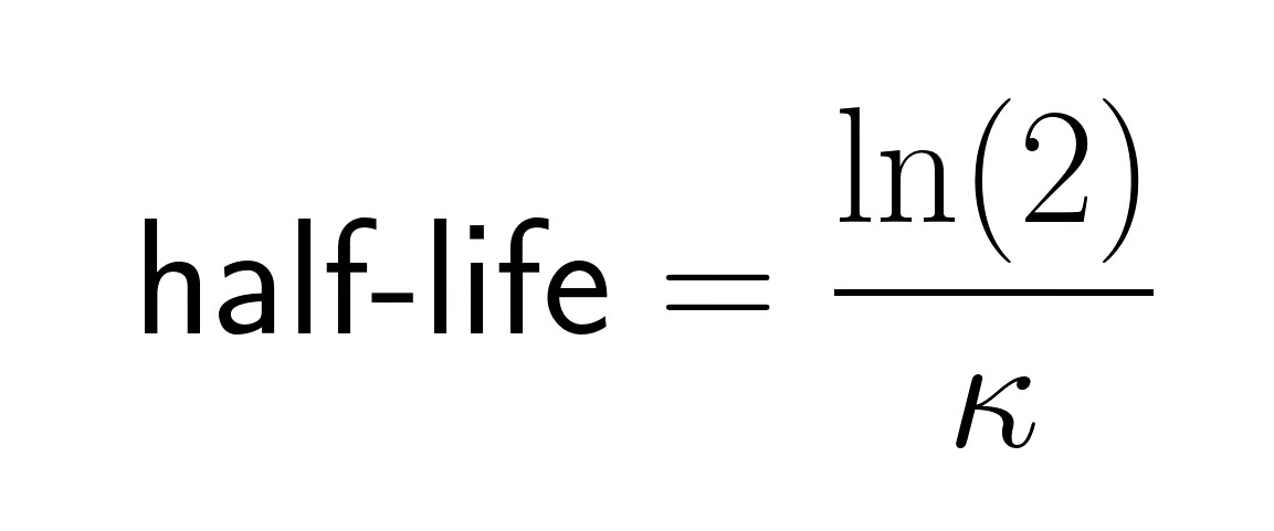
A half-life of three days means the process is rapid; deviations collapse within a week. A half-life of six months means you'd need a long holding period to capture the reversion, which creates its own risks. Quant traders compare estimated half-lives against their target holding periods before committing to a strategy.

One caution: the half-life is an expected value, not a guarantee. Any given deviation could persist much longer, especially around regime changes or structural breaks.

Mean Reversion in Finance

Where does mean reversion actually show up in financial markets? In some places the evidence is solid; in others, less so.

• Asset spreads. Spreads between related assets (the price difference between two stocks in the same sector, or the yield spread between two similar bonds) are among the most plausible candidates for mean reversion. Neither individual price needs to be stationary; the spread between them can be, if the assets share a long-run relationship.
• Interest rates. Short-term interest rates show historically strong mean-reverting behavior. Central banks have target ranges, and rates that move too far from them tend to get pulled back by policy. Longer-term rates are more debated.
• Volatility. Implied and realized volatility are widely understood to be mean-reverting. Volatility spikes, like those seen during March 2020, are dramatic but temporary. The VIX eventually returns to more normal levels, and volatility traders routinely exploit this.
• Valuation ratios. Price-to-earnings ratios, price-to-book ratios, and similar metrics show long-run mean reversion, though the "long run" can be very long indeed. Relying on valuation mean reversion over short horizons is a well-documented source of early losses.
• Commodity prices. Commodity prices (oil, natural gas, agricultural products) are often modeled as mean-reverting to long-run marginal cost of production. When prices spike well above production cost, new supply comes online; when they crash below, supply contracts. The mechanism is real, but so is the uncertainty about where the "true" mean sits at any given time.

One thing worth flagging: individual equity prices are generally non-stationary. It's spreads, returns, volatility measures, or other transformations that tend to show mean-reverting behavior, not raw price levels.

Mean Reversion, Correlation, and Cointegration

There's yet another conceptual distinction that trips up even experienced people in this space, and getting it wrong leads to poorly constructed strategies.

• Correlation measures how two variables move together. High correlation means they tend to rise and fall at the same time. But it says nothing about whether the spread between them is mean-reverting. Two stocks can have a correlation of 0.9 and still make a poor pairs trade, because correlation tells you nothing about whether the spread between them is stable over time.
• Cointegration is a stronger statement. Two non-stationary series are cointegrated if a linear combination of them is stationary, meaning they share a long-run equilibrium relationship and can't drift apart permanently. Both stocks can trend upward together for years, then diverge permanently: that's high correlation with no cointegration, and no reliable trade. Testing for cointegration using the Engle-Granger test or the Johansen procedure gives you a more defensible basis for assuming the spread will revert. This is the statistical foundation for pairs trading.

You can have two assets with 0.95 correlation whose spread is a random walk. Always test.

Mean Reversion and Pairs Trading

Pairs trading is the clearest example of mean reversion put to practical use, and you might have landed on this article because of that connection.

You start by identifying two assets with a plausible long-run economic relationship: two oil majors, two large-cap banks, two consumer staples companies. The economic rationale matters here. Screening purely on historical correlations without a fundamental basis tends to produce spurious relationships that fall apart out of sample. You construct a spread, typically a ratio or a linear combination of the two prices, using a hedge ratio estimated from regression rather than a naïve one-to-one assumption. Then you test whether that spread is mean-reverting using the tools covered above: the ADF test, autocorrelation analysis, half-life estimation. If the evidence is supportive, you proceed.

The trade itself is fairly straightforward. When the spread widens unusually far from its historical mean, measured using a z-score that standardizes the deviation as (current spread minus moving mean) divided by standard deviation, you go long the underperformer and short the outperformer, expecting the spread to narrow. A z-score of +2 signals the spread is two standard deviations above its historical norm; a common approach is to enter at ±2.0 and exit when it reverts toward zero. The key point, one that gets lost in simpler explanations: it's the spread that's expected to mean-revert, not either individual stock. The long/short structure also reduces exposure to broad market movements. The profit comes from the relative move, not market direction.

Statistical Arbitrage: Taking It Further

Pairs trading is the most intuitive entry point into mean reversion strategies, but it's one instance of a broader family of approaches known as statistical arbitrage.

Statistical arbitrage (stat arb) uses statistical relationships between securities to spot relative mispricing: when two historically linked securities temporarily diverge from their expected relationship, you bet they'll converge. One important clarification: statistical arbitrage is not risk-free arbitrage. Traditional arbitrage exploits near-mechanical price discrepancies, the same asset trading at different prices on two exchanges, where the profit is close to certain if you can execute fast enough. Statistical arbitrage bets on probabilistic convergence. Entirely different risk profiles.

Mean Reversion Trading Strategies

There are different mean reversion trading ideas. Here are some of them:

• Z-score strategies. Standardize deviations from a rolling historical mean by the rolling standard deviation. A z-score above +2 signals the variable is unusually extended; below −2 signals it's unusually depressed. Trading based on z-score thresholds is one of the simplest implementations of mean reversion and is widely used for single assets, spreads, and factor portfolios.
• Bollinger Band strategies. Bollinger Bands place upper and lower envelopes around a moving average, at two standard deviations. When price touches the upper band, the series is extended relative to recent history; when it touches the lower band, it's depressed. The strategy trades the expected return toward the moving average. Keep in mind that the moving average is the "mean" being reverted to, so the relevant question is always whether a given asset actually mean-reverts, not just whether it touches the band.
• Pairs trading. Already covered above. The spread is the object of interest, and the position is market-neutral by construction.
• Multi-asset statistical arbitrage. The same logic as pairs trading, extended to portfolios of many assets. You're doing principal component analysis on a large covariance matrix, but the intuition is the same.

Worth saying plainly: a statistical signal doesn't guarantee profitable convergence. Transaction costs, borrowing costs, and regime changes can wipe out apparent edges entirely. The strategies above describe conditions for entering a position, not conditions for making money.

How to Analyze Mean Reversion in Python

Here's where things get practical. The code below walks through a compact mean-reversion analysis on a simulated spread, covering the essentials: plotting, rolling mean, ADF test, and half-life estimation. Swap in a real pairs spread, say the log price ratio of two cointegrated stocks, and the same pipeline applies.

import numpy as np
import pandas as pd
import matplotlib.pyplot as plt
from statsmodels.tsa.stattools import adfuller
from statsmodels.regression.linear_model import OLS

# Simulate a mean-reverting spread using an AR(1) process
np.random.seed(42)
n = 500
phi = 0.92          # AR coefficient; close to 1 = slow mean reversion
spread = np.zeros(n)
for t in range(1, n):
    spread[t] = phi * spread[t-1] + np.random.normal(0, 1)

spread_series = pd.Series(spread, name="spread")

# --- Step 1: Plot the series with its rolling mean ---
rolling_mean = spread_series.rolling(window=60).mean()
plt.figure(figsize=(10, 4))
plt.plot(spread_series, label="Spread", alpha=0.7)
plt.plot(rolling_mean, label="60-period rolling mean", linewidth=2)
plt.axhline(0, color="black", linestyle="--", linewidth=0.8)
plt.title("Simulated Mean-Reverting Spread")
plt.legend()
plt.tight_layout()
plt.show()

# --- Step 2: ADF test for stationarity ---
adf_result = adfuller(spread_series.dropna())
print(f"ADF statistic : {adf_result[0]:.4f}")
print(f"p-value       : {adf_result[1]:.4f}")
print("Reject unit root?", "Yes" if adf_result[1] < 0.05 else "No")

# --- Step 3: Estimate half-life via AR(1) regression —
lagged = spread_series.shift(1).dropna()
delta  = spread_series.diff().dropna()
model  = OLS(delta, lagged).fit()
kappa  = -model.params.iloc[0]           # speed of mean reversion
half_life = np.log(2) / kappa
print(f"\nEstimated half-life: {half_life:.1f} periods")

Running this with the seed above gives a p-value well below 0.05 and a half-life of roughly seven periods. The theoretical value for φ = 0.92 is about 8.7 periods; individual runs will vary around that. Just remember: interpretation matters more than the mechanics. A statistically significant ADF result on a historical window doesn't mean the relationship will hold going forward. This regression omits an intercept, which is valid for zero-mean data. For real spreads with a non-zero mean, add a constant using add_constant(lagged) and extract the second coefficient.

Our Time Series Analysis in Python course goes much deeper on these techniques, including ARIMA modeling, stationarity testing, and forecasting.

Risks and Limitations of Mean Reversion

Mean reversion fails in predictable ways. Knowing the failure modes is as useful as knowing the strategy.

The mean can change

Historical equilibrium levels are estimated from data, and data reflects the past. Structural breaks (a merger, a regulatory change, a shift in competitive dynamics) can invalidate the historical mean entirely. The spread you thought was mean-reverting to zero may now have an equilibrium at +50 basis points. Applying a strategy built on the old mean is a reliable way to lose money. In pairs trading specifically, companies merge, diverge, or change their business models, and a pair that was tightly cointegrated for five years can decouple overnight.

Trends can be mistaken for mean reversion

Over a short sample, a trending series can look mean-reverting simply because it reverts to a local moving average. This is especially common in backtests that use a fixed lookback window. The fix is to test across multiple sample periods and to be skeptical of results that only appear over narrow windows.

Transaction costs

Frequent trading eats into returns. A strategy with a two-day half-life might require daily rebalancing, and round-trip transaction costs can easily exceed the expected profit per trade. Shorting adds further costs: securities lending fees and the risk of being bought in by a broker. Slippage between modeled and actual fill prices accumulates across hundreds of trades. Paper returns and live returns can differ dramatically for high-frequency mean-reversion strategies.

Crowded trades

When many funds run similar strategies, they become exposed to each other's behavior. The August 2007 quant meltdown happened precisely because too many equity stat arb funds liquidated simultaneously, and the resulting cascade had nothing to do with the underlying relationships those strategies were built on. When a strategy works, it attracts capital; when it attracts too much capital, it stops working, sometimes gradually and sometimes all at once.

Regime changes

Stat arb models are calibrated to a particular market environment: a volatility regime, an interest rate cycle, a correlation structure. When that environment shifts, every assumption moves at once. It's not one pair breaking down; it's the entire portfolio misbehaving because the statistical properties it was built on no longer hold. Historical lookback windows won't warn you in advance.

Parameter sensitivity

Results depend heavily on the lookback window used to estimate the mean, the threshold for entering trades, and the exit rule. Small changes to any of these can flip a strategy from profitable to unprofitable. Stress-test this explicitly before trusting any backtest.

Backtest overfitting

The most insidious risk. With enough parameters and historical data, you can fit a strategy to almost any past period, and it will degrade sharply in live trading. Walk-forward testing and out-of-sample validation aren't optional.

Conclusion

Mean reversion is one of those concepts that sounds simple until you try to use it. The basic idea, that deviations from equilibrium tend to reverse, is intuitive. What's harder is establishing whether a particular series actually has that property, estimating how quickly it reverts, and building strategies that survive transaction costs, regime changes, and parameter uncertainty. Statistical arbitrage formalizes that challenge into a trading discipline, but the core difficulty stays the same: the relationships you're trading are competing with everyone else who found the same ones.

A few things to take away: test before you assume; pay attention to what's doing the reverting (spreads and transformations, not raw prices); distinguish correlation from cointegration, because they're not interchangeable; and treat the risks above as part of the strategy, not an afterthought. Our Time Series Analysis in Python course covers stationarity testing, ARIMA modeling, and forecasting in depth. For trading applications specifically, Financial Trading in Python covers implementing and evaluating quantitative strategies in practice.