Verlaufs- und Dichteplots in R

Du kannst Histogramme mit der Funktion hist(x</em>) erstellen, wobei x ein numerischer Vektor von Werten ist, die gezeichnet werden sollen. Mit der Option freq=FALSE werden Wahrscheinlichkeitsdichten anstelle von Häufigkeiten gezeichnet. Die Option breaks= bestimmt die Anzahl der Bins.

# Simple Histogram
hist(mtcars$mpg)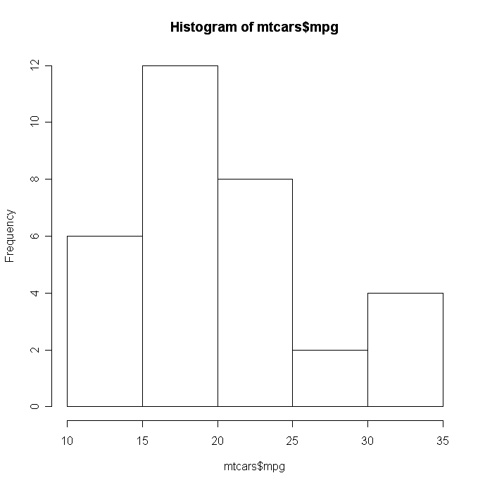

# Colored Histogram with Different Number of Bins
hist(mtcars$mpg, breaks=12, col="red")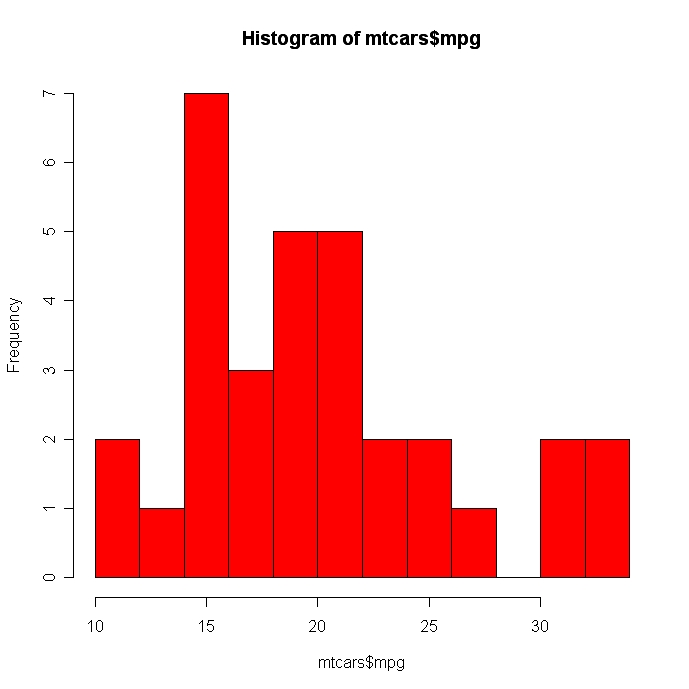

# Add a Normal Curve (Thanks to Peter Dalgaard)
x <- mtcars$mpg
h<-hist(x, breaks=10, col="red", xlab="Miles Per Gallon",
   main="Histogram with Normal Curve")
xfit<-seq(min(x),max(x),length=40)
yfit<-dnorm(xfit,mean=mean(x),sd=sd(x))
yfit <- yfit*diff(h$mids[1:2])*length(x)

lines(xfit, yfit, col="blue", lwd=2)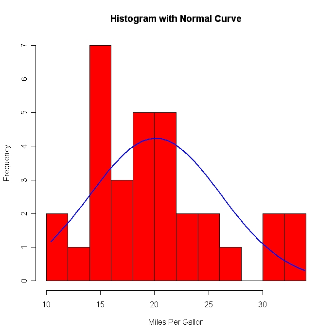

Histogramme können eine schlechte Methode sein, um die Form einer Verteilung zu bestimmen, weil sie so stark von der Anzahl der verwendeten Bins beeinflusst wird.

Kernel-Dichte-Diagramme

Kerndichtediagramme sind in der Regel eine viel effektivere Methode, um die Verteilung einer Variablen zu betrachten. Erstelle den Plot mit plot(density(x)), wobei x ein numerischer Vektor ist.

# Kernel Density Plot
d <- density(mtcars$mpg) # returns the density data
plot(d) # plots the results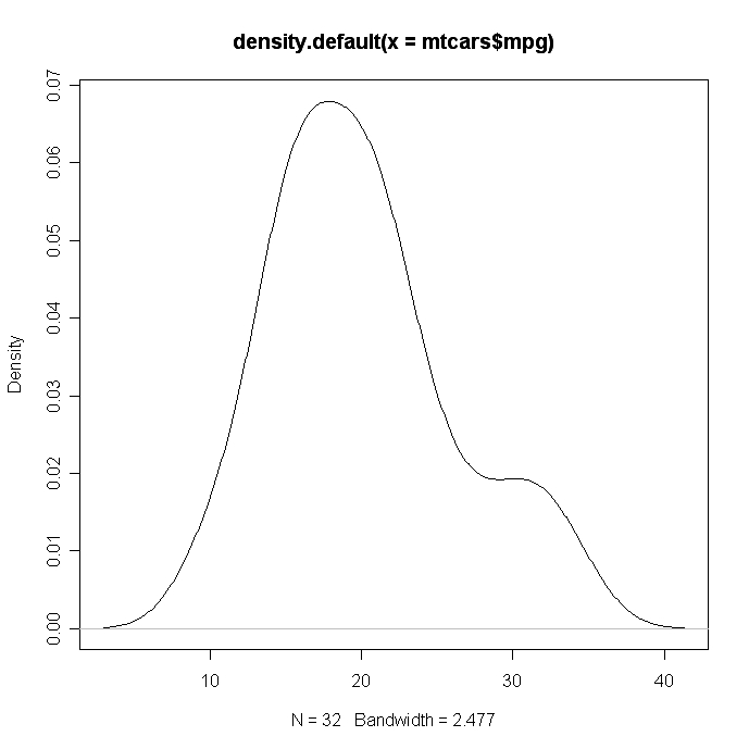

# Filled Density Plot
d <- density(mtcars$mpg)
plot(d, main="Kernel Density of Miles Per Gallon")
polygon(d, col="red", border="blue")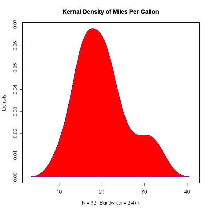

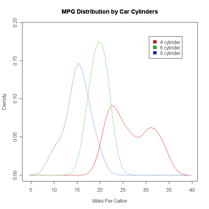
Gruppenvergleich VIA-Kernel-Dichte

Mit der Funktion sm.density.compare( ) im Paket sm</a ></strong > kannst du die Kerndichtediagramme von zwei oder mehr Gruppen übereinanderlegen. Das Format ist sm.density.compare(x , factor), wobei x ein numerischer Vektor und factor die Gruppierungsvariable ist.

# Compare MPG distributions for cars with
#
4,6, or 8 cylinders
library(sm)
attach(mtcars)

# create value labels
cyl.f <- factor(cyl, levels= c(4,6,8),
  labels = c("4 cylinder", "6 cylinder", "8 cylinder"))

# plot densities
sm.density.compare(mpg, cyl, xlab="Miles Per Gallon")
title(main="MPG Distribution by Car Cylinders")

# add legend via mouse click
colfill<-c(2:(2+length(levels(cyl.f))))
legend(locator(1), levels(cyl.f), fill=colfill)